

Creating DTC Glaciers User-DT-Enhanced Data cubes (L3)#
A central aspect that distinguishes DTC Glaciers as a Digital Twin Component is that users are not limited to downloading pre-computed products. Instead, the system supports active interaction, where users can integrate their own data into the workflow.
This notebook introduces Level 3 (L3) data cubes: user-driven, model–data cubes generated by combining user-provided datasets with the DTC Glaciers modelling and assimilation framework. L3 data cubes extend the pre-computed L1 and L2 products by enabling users to explore alternative data sources, assumptions, or scenarios within the same Digital Twin architecture.
In this notebook, we demonstrate how users can provide their own observational or derived data, generate corresponding L3 data cubes, and subsequently validate these against existing DTC Glaciers products. This includes direct comparison with pre-computed L2 data cubes, as well as validation using user-supplied observations.
The workflow illustrated here highlights how DTC Glaciers supports experimentation, hypothesis testing, and application-specific analyses, whilst maintaining consistency with the underlying DTC framework.
If required, install the DTCG API using the following command:
!pip install 'dtcg[jupyter] @ git+https://github.com/DTC-Glaciers/dtcg'
Run this command in a notebook cell.
# Imports
import dtcg.integration.oggm_bindings as oggm_bindings
import dtcg.integration.calibration as calibration
from dtcg import DEFAULT_L2_DATACUBE_URL

from oggm.core import massbalance

import matplotlib.pyplot as plt
import numpy as np
Preparing the scene#
In this example, we focus on Iceland, where we have example in-situ mass balance data from the National Power Company of Iceland, Landsvirkjun, a key stakeholder of DTC Glaciers.
We concentrate on Brúarjökull, an outlet glacier of Vatnajökull, the largest ice cap in Iceland. In the following cells, we open the example data and reproject it onto the same grid as our data cubes.
rgi_id_ice = "RGI60-06.00377"  # Brúarjökull
dtcg_oggm_ice = oggm_bindings.BindingsOggmModel(rgi_id=rgi_id_ice)


def get_l2_data_tree(rgi_id):
    return xr.open_datatree(
        f"{DEFAULT_L2_DATACUBE_URL}{rgi_id}.zarr",
        chunks={},
        engine="zarr",
        consolidated=True,
        decode_cf=True,
    )


data_tree_ice = get_l2_data_tree(rgi_id_ice)
# add user data
from oggm import workflow

workflow.execute_entity_task(add_iceland_smb, dtcg_oggm_ice.gdir)

# open user data
with xr.open_dataset(dtcg_oggm_ice.gdir.get_filepath("iceland_smb")) as ds_user:
    ds_user = ds_user
ds_user
<xarray.Dataset> Size: 112MB
Dimensions:  (time_a: 29, y: 370, x: 436, time: 58)
Coordinates:
  * time_a   (time_a) datetime64[ns] 232B 1996-10-01 1997-10-01 ... 2024-10-01
  * y        (y) float32 1kB 7.201e+06 7.201e+06 ... 7.127e+06 7.127e+06
  * x        (x) float32 2kB 3.94e+05 3.942e+05 3.944e+05 ... 4.808e+05 4.81e+05
  * time     (time) datetime64[ns] 464B 1996-05-01 1996-10-01 ... 2024-10-01
Data variables:
    ba       (time_a, y, x) float64 37MB ...
    b        (time, y, x) float64 75MB ...
Attributes:
pyproj_srs: +proj=utm +zone=28 +datum=WGS84 +units=m +no_defsLet’s take a first look at the gridded data and the mean annual mass balance:
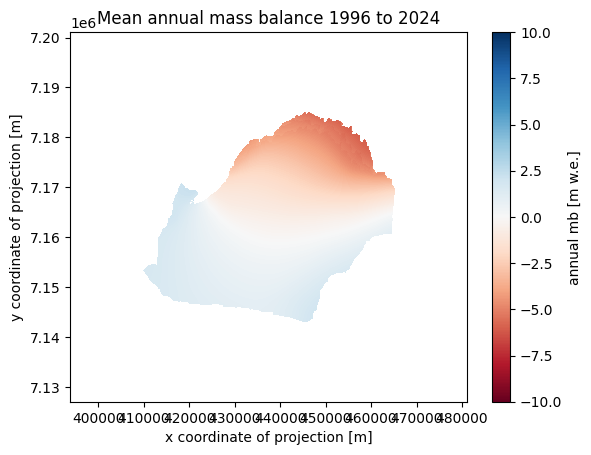
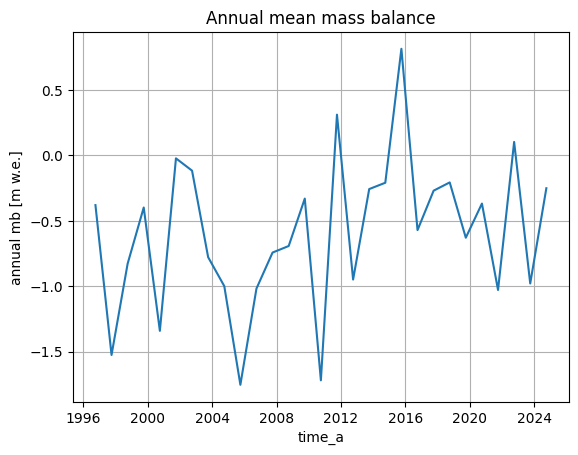
annual_smb = ds_user["ba"].where(dtcg_oggm_ice.datacube_l1.glacier_mask)
avg_smb = annual_smb.mean(dim="time_a", keep_attrs=True)
avg_smb.plot(cmap="RdBu", vmin=-10, vmax=10)
plt.title("Mean annual mass balance 1996 to 2024")
plt.show()

annual_smb.mean(dim=("y", "x")).plot()
plt.grid("on")
plt.title("Annual mean mass balance")
plt.show()
Create L3 data cubes#
DTC Glaciers makes it easy for users to interact with the system and generate custom model output, rather than relying only on preprocessed, static results. Here, we demonstrate a first use case in which a user can provide their own observations, generate L3 data cubes, and further use their own data for validation (shown in one of the next sections).
Let’s prepare the user data as cumulative mass balance for the period 2010–2020:
def get_date_string(date):
    return np.datetime_as_string(date, unit="D").item()


start_date = annual_smb.time_a[14].values  # 2010
end_date = annual_smb.time_a[24].values  # 2020

# the period of the reference mass balance, e.g. '2010-01-01_2020-01-01'
ref_mb_period = f"{get_date_string(start_date)}_" f"{get_date_string(end_date)}"

# the actual observation value calculated as the cumulative mass balance over the period of interest
annual_cumsum_smb = annual_smb.mean(dim=("y", "x")).cumsum()
ref_mb = (
    annual_cumsum_smb.sel(time_a=end_date).values
    - annual_cumsum_smb.sel(time_a=start_date).values
) * 1000  # convert to mm w.e., which is equal to kg m-2

# the unit of the provided observation
ref_mb_unit = "kg m-2"

# an associated uncertainty, in this example we just set a typical order of magnitude
ref_mb_err = 500

# this description is add to the attributes of the resulting datacubes for reference
calibration_strategy = (
    "OGGM model DailyTIModel calibrated with user data "
    f"from Landsvirkjun over the period {ref_mb_period}."
)

# this is the name which will be used when adding the datacube to a datatree
l3_datacube_name = (
    f"L3_Daily_Landsvirkjun_"
    f"{get_date_string(start_date).split('-')[0]}_"
    f"{get_date_string(end_date).split('-')[0]}"
)
Currently, DTC Glaciers supports calibration of the mass balance only over a complete reference period. However, in OGGM it is also possible to calibrate using an incomplete set of mass balance observations, for example by considering only selected years. This functionality could potentially be added to DTC Glaciers in the future.
Now we provide the user data to the calibrator and create L3 data cubes. For this, we use calibrator.calibrate_mb_and_create_datacubes, which takes as input the mass balance model to be calibrated and the reference mass balance values:
calibrator = calibration.CalibratorCryotempo(
    datacube_l1=data_tree_ice["L1"].ds, gdir=dtcg_oggm_ice.gdir
)

l3_datacubes = calibrator.get_calibrated_datacubes(
    mb_model_class=massbalance.DailyTIModel,
    ref_mb=ref_mb,
    ref_mb_err=ref_mb_err,
    ref_mb_unit=ref_mb_unit,
    ref_mb_period=ref_mb_period,
    calibration_strategy=calibration_strategy,
    datacube_types=["monthly", "annual_hydro", "daily_smb"],
    show_log=True,  # to see what is happening
    # we set here a small ensemble number for MCS for demonstration to reduce computing time,
    # the precomputed datacubes use 2**4~100 ensemble members
    mcs_sampling_settings={"nr_samples": 2**1},
)
DailyTIModel_2010-10-01_2020-10-01:
  Starting Monte Carlo Simulation for 12 ensemble members.
  Finished Monte Carlo Simulation: 12 ensemble members for output aggregation available.
  Start generating datacubes
    Start generation of monthly datacube
    Finished generation of monthly datacube
    Start generation of annual_hydro datacube
    Finished generation of annual_hydro datacube
    Start generation of daily_smb datacube
    Finished generation of daily_smb datacube
  Finished generating datacubes
The resulting L3 data cube can be added to the existing data_tree in the same way as the L2 data cubes:
from dtcg.datacube.geozarr import GeoZarrHandler

datacube_handler = GeoZarrHandler(ds=data_tree_ice)

datacube_handler.add_datacube(datacubes=l3_datacubes, datacube_name=l3_datacube_name)

list(datacube_handler.data_tree.keys())
['L1',
 'L2_Daily_Cryosat_2011_2020',
 'L2_Daily_Hugonnet_2000_2020',
 'L2_Daily_Hugonnet_2010_2020',
 'L2_SfcDaily_Cryosat_2011_2020',
 'L3_Daily_Landsvirkjun_2010_2020']

# datacube_handler.export('datacube_including_L3.zarr')
Validate L3 data cubes#
The general validation of L3 data cubes works in the same way as for L2, as explained in this notebook. Let’s have a look:
# select the datacubes which should be evaluated
validation_name_list = [
    "L2_Daily_Cryosat_2011_2020",
    "L2_Daily_Hugonnet_2010_2020",
    "L3_Daily_Landsvirkjun_2010_2020",
]
from dtcg.validation.validator import DatacubeValidator

# conduct the actual validation
validator = DatacubeValidator(datacube_handler.data_tree)
validation_data = validator.get_validation_for_layers(l2_name_list=validation_name_list)
validation_data["WGMS"]
| MeanAbsD (mm w.e. yr-1) | MeanD (mm w.e. yr-1) | MedianD (mm w.e. yr-1) | RMSD (mm w.e. yr-1) | CORRCOEF | |
|---|---|---|---|---|---|
| L1 WGMS annual mass balance 2000-2024 | |||||
| L2_Daily_Cryosat_2011_2020 | 415.9 (346.9, 501.2) | 9.7 (-138.7, 187.5) | 3.0 (-131.5, 169.7) | 530.2 (440.1, 630.6) | 0.49 (0.28, 0.72) |
| L2_Daily_Hugonnet_2010_2020 | 513.2 (373.5, 637.9) | -294.6 (-445.3, -110.7) | -308.1 (-476.3, -121.3) | 621.2 (477.0, 754.4) | 0.48 (0.24, 0.70) |
| L3_Daily_Landsvirkjun_2010_2020 | 441.5 (335.6, 536.7) | -124.1 (-267.2, 61.2) | -135.4 (-265.4, 42.1) | 551.5 (434.8, 658.4) | 0.49 (0.27, 0.71) |
validation_data["CryoSat2"]
| MeanAbsD (m) | MeanD (m) | MedianD (m) | RMSD (m) | CORRCOEF | |
|---|---|---|---|---|---|
| L1 CryoSat2 elevation change 2011-01-01_2025-09-01 | |||||
| L2_Daily_Cryosat_2011_2020 | 0.6 (0.5, 0.8) | -0.0 (-0.3, 0.2) | -0.0 (-0.4, 0.3) | 0.7 (0.7, 0.9) | 0.88 (0.71, 0.89) |
| L2_Daily_Hugonnet_2010_2020 | 2.9 (2.1, 3.6) | -2.9 (-3.6, -2.0) | -3.6 (-3.7, -1.3) | 3.4 (2.8, 4.1) | 0.83 (0.58, 0.82) |
| L3_Daily_Landsvirkjun_2010_2020 | 1.4 (1.0, 1.7) | -1.2 (-1.6, -0.8) | -1.5 (-1.7, -0.7) | 1.6 (1.3, 1.9) | 0.86 (0.67, 0.89) |
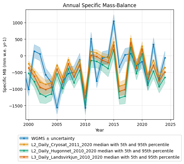
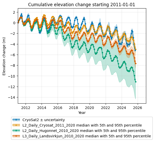
We see that the L3 data cube lies somewhere between the two L2 data cubes calibrated with Hugonnet et al. (2021) and CryoSat-2 data. This is also confirmed by a visual comparison of the results in the plot:
validator.get_validation_plot_for_layers(
    l2_name_list=validation_name_list, obs_name="WGMS"
)
plt.show()
validator.get_validation_plot_for_layers(
    l2_name_list=validation_name_list, obs_name="CryoSat2"
)
plt.show()
Validation with user data#
Another level of interaction between the user and DTC Glaciers is the ability to bring your own data and use the tools of the validation framework to evaluate the supported validation metrics or to create plots for visually inspecting differences.
For this, we need to format the user data as follows:
annual_mb = annual_smb.mean(dim=("y", "x"))

user_observation = {
    # Let the validation framework know which type of observation is provided
    "obs_type": "annual_mb",
    # The observed values
    "values": annual_mb.values * 1000,
    # Corresponding uncertainties
    "uncertainty": np.full(annual_mb.values.shape, 200),
    # The observation years
    "years": np.array(
        [
            yr.astype("datetime64[Y]").astype(int) + 1970
            for yr in annual_mb.time_a.values
        ]
    ),
    # Name of the data source (displayed in the validation tables)
    "name": "Landsvirkjun provided annual mass balance",
}
Once the data is prepared, provide it via user_observation and interact with the validation framework in the same way as before:
validation_data, bootstrap_args = validator.get_validation_for_layers(
    user_observation=user_observation,
    l2_name_list=validation_name_list,
    return_bootstrap_args=True,
)
validation_data["annual_mb"]
| MeanAbsD (mm w.e. yr-1) | MeanD (mm w.e. yr-1) | MedianD (mm w.e. yr-1) | RMSD (mm w.e. yr-1) | CORRCOEF | |
|---|---|---|---|---|---|
| Landsvirkjun provided annual mass balance 2000-2024 | |||||
| L2_Daily_Cryosat_2011_2020 | 474.1 (408.9, 540.6) | 226.9 (86.7, 394.8) | 192.5 (63.0, 406.9) | 579.6 (489.3, 678.5) | 0.48 (0.26, 0.72) |
| L2_Daily_Hugonnet_2010_2020 | 443.5 (337.5, 548.0) | -77.4 (-222.0, 97.7) | -110.7 (-282.5, 106.5) | 555.5 (435.6, 668.5) | 0.47 (0.23, 0.70) |
| L3_Daily_Landsvirkjun_2010_2020 | 440.6 (363.5, 511.7) | 93.1 (-43.0, 269.6) | 55.7 (-70.5, 280.5) | 548.5 (449.3, 645.9) | 0.48 (0.26, 0.72) |
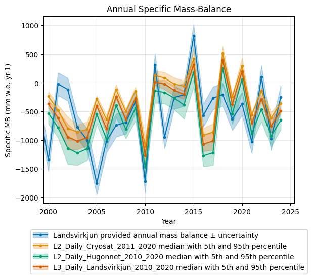
In this case, we see that the newly generated L3 data cube performs slightly better than the other two options. This is expected, as parts of the user-provided data were also used for calibration, and the validation is therefore not fully independent.
You can also provide the user_observation to the plotting functions to visually compare different data cubes with the provided observations:
validator.get_validation_plot_for_layers(
    user_observation=user_observation, l2_name_list=validation_name_list
)
plt.show()