Validating DTC Glaciers EO-DT-Enhanced Data Cubes (L2)

To assess the performance of different L2 data cubes, this notebook illustrates the capabilities of the DTC Glaciers validation framework.
The objective is to evaluate L2 data cubes by comparing their model-derived estimates against independent observations available from the corresponding L1 data cubes.

This validation step is a core component of the DTC Glaciers concept, providing a transparent way to quantify consistency between observations and model-based reconstructions, and to characterise associated uncertainties.

We begin by opening two examples from the pre-processed L2 data cubes:

If required, install the DTCG API using the following command:

!pip install 'dtcg[jupyter] @ git+https://github.com/DTC-Glaciers/dtcg'

Run this command in a notebook cell.

# Imports
import xarray as xr
import matplotlib.pyplot as plt

from dtcg import DEFAULT_L2_DATACUBE_URL

rgi_id_ice = "RGI60-06.00377"  # Brúarjökull
rgi_id_aut = "RGI60-11.00719"  # Vernagtferner


def get_l2_data_tree(rgi_id):
    return xr.open_datatree(
        f"{DEFAULT_L2_DATACUBE_URL}{rgi_id}.zarr",
        chunks={},
        engine="zarr",
        consolidated=True,
        decode_cf=True,
    )


data_tree_ice = get_l2_data_tree(rgi_id_ice)
data_tree_aut = get_l2_data_tree(rgi_id_aut)

Validation of DTC Glaciers output

The validation within DTC Glaciers consists of a combination of in-situ observations and Earth observation (EO) data from the L1 data cubes. The entire validation framework is built around the DatacubeValidator, which only requires a data tree as input:

from dtcg.validation.validator import DatacubeValidator

validator_ice = DatacubeValidator(data_tree_ice)
validator_aut = DatacubeValidator(data_tree_aut)

We assess the performance of different L2 data cubes with respect to observations by calculating the following metrics:

validator_ice.get_description_of_metrics()

{'MeanAbsD': 'Mean Absolute Deviation',
 'MeanD': 'Mean Deviation',
 'MedianD': 'Median Deviation',
 'RMSD': 'Root Mean Squared Deviation',
 'CORRCOEF': 'Pearson correlation coefficient'}

To account for observation and model uncertainty during validation, we rely on bootstrapping. For this purpose, the performance metrics are not only evaluated for the most likely observation and model values, but we also generate a distribution for each metric.

This is done by repeatedly resampling the time series in coherent multi-year blocks and drawing a plausible value for each resampled year from the corresponding uncertainty description. For observations, we assume a normal distribution, while the model output is represented by seven quantiles (0.05, 0.15, 0.25, 0.5, 0.75, 0.85, and 0.95).

By default, this procedure is repeated 5,000 times. The resulting sampling distribution is then summarised using a 90% confidence interval, which is shown in brackets in the validation output below.

Below, we show two examples of the validation framework for our two case study regions, which differ in their data availability.

Iceland

In Iceland, we have Earth observation data from CryoTEMPO-EOLIS (CryoSat-2), as well as in-situ observations from WGMS for some glaciers.

Let’s see which L2 data cubes are available:

list(data_tree_ice.keys())

['L1',
 'L2_Daily_Cryosat_2011_2020',
 'L2_Daily_Hugonnet_2000_2020',
 'L2_Daily_Hugonnet_2010_2020',
 'L2_SfcDaily_Cryosat_2011_2020']

For the following analysis, we selected the daily mass balance model calibrated with CryoTEMPO-EOLIS (CryoSat-2) for the period 2011–2020. We then compared it to the same model calibrated with Hugonnet et al. (2021) for the period 2010–2020.

l2_list_ice = ["L2_Daily_Cryosat_2011_2020", "L2_Daily_Hugonnet_2010_2020"]

With the DatacubeValidator already set up, we only need to provide the L2 data cubes of interest. The validator then checks which reference data are available in the L1 data cubes and computes the corresponding performance metrics.

validation_data_ice, bootstrap_args_ice = validator_ice.get_validation_for_layers(
    l2_name_list=l2_list_ice, return_bootstrap_args=True
)

Let’s start by examining the results of comparing the L2 data cubes with the CryoSat-2 observations:

validation_data_ice["CryoSat2"]

	MeanAbsD (m)	MeanD (m)	MedianD (m)	RMSD (m)	CORRCOEF
L1 CryoSat2 elevation change 2011-01-01_2025-09-01
L2_Daily_Cryosat_2011_2020	0.6 (0.5, 0.8)	-0.0 (-0.3, 0.2)	-0.0 (-0.4, 0.3)	0.7 (0.7, 0.9)	0.88 (0.71, 0.89)
L2_Daily_Hugonnet_2010_2020	2.9 (2.1, 3.6)	-2.9 (-3.6, -2.0)	-3.6 (-3.7, -1.3)	3.4 (2.8, 4.1)	0.83 (0.58, 0.82)

We see that the data cube calibrated with CryoSat-2 outperforms the one calibrated with Hugonnet et al. (2021).
The metrics that quantify absolute differences (MeanAbsD, RMSD) show smaller values, indicating a better overall agreement.

Metrics that quantify bias (MeanD and MedianD) are closer to zero, and their confidence intervals span both positive and negative values, suggesting no strong systematic bias. Finally, the correlation coefficient is higher, indicating a stronger linear relationship between the observations and the model output.

To help with interpretation, we can also take a look at the bootstrap settings used during the validation:

bootstrap_args_ice["CryoSat2"]

{'ci_level': 0.9, 'n': 177, 'n_boot': 5000, 'block_length': 13, 'seed': 0}

We see that the reported metric intervals correspond to a 90% confidence interval (ci_level). In total, 173 observations are available (n). The validation is based on 5,000 bootstrap resamplings of the time series and repeated evaluations of the metrics (n_boot). A block length of 13 observations was used to preserve temporal coherence (block_length). For reproducibility, a fixed random seed is applied.

However, it is important to note that this validation is not fully independent, because the CryoSat-2 data cube uses part of the same data for calibration. Therefore, we also evaluate the model performance using independent data only by defining a dedicated validation period:

validation_cryosat_2020_2025 = validator_ice.get_validation_for_layers(
    l2_name_list=l2_list_ice,
    baseline_date="2020-01-01",  # the date where the cumulated elevation change starts
    obs_list=[
        "CryoSat2"
    ],  # we can select to only perform the validation on one observation
    validation_period="2020-01-01_2025-12-31",
)  # define the period which should be considered

validation_cryosat_2020_2025["CryoSat2"]

	MeanAbsD (m)	MeanD (m)	MedianD (m)	RMSD (m)	CORRCOEF
L1 CryoSat2 elevation change 2020-01-01_2025-09-01
L2_Daily_Cryosat_2011_2020	0.6 (0.5, 0.7)	0.4 (0.2, 0.6)	0.4 (0.2, 0.6)	0.7 (0.6, 0.9)	0.93 (0.78, 0.91)
L2_Daily_Hugonnet_2010_2020	0.8 (0.6, 1.2)	-0.7 (-1.1, -0.4)	-0.6 (-1.0, -0.3)	1.0 (0.8, 1.5)	0.89 (0.66, 0.87)

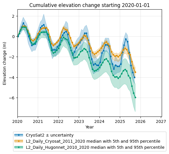
Even when using the independent validation period, the CryoSat-2–calibrated data cube still outperforms the Hugonnet-calibrated data cube. However, the differences are less pronounced than when using the full time period.

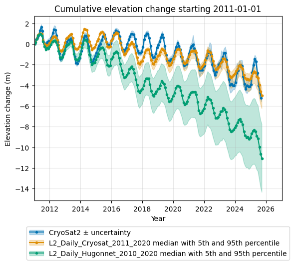
We can also use the DatacubeValidator to gain a visual impression of model performance by creating comparison plots.

First, for the entire period:

validator_ice.get_validation_plot_for_layers(
    l2_name_list=l2_list_ice, obs_name="CryoSat2"
)
plt.show()

Or for the independent validation period, by defining a baseline_date:

fig = validator_ice.get_validation_plot_for_layers(
    l2_name_list=l2_list_ice, obs_name="CryoSat2", baseline_date="2020-01-01"
)
plt.show()

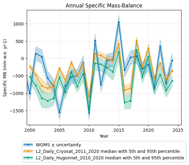
Another available data source for our test glacier is in-situ mass balance observations from WGMS:

validation_data_ice["WGMS"]

	MeanAbsD (mm w.e. yr-1)	MeanD (mm w.e. yr-1)	MedianD (mm w.e. yr-1)	RMSD (mm w.e. yr-1)	CORRCOEF
L1 WGMS annual mass balance 2000-2024
L2_Daily_Cryosat_2011_2020	415.9 (346.9, 501.2)	9.7 (-138.7, 187.5)	3.0 (-131.5, 169.7)	530.2 (440.1, 630.6)	0.49 (0.28, 0.72)
L2_Daily_Hugonnet_2010_2020	513.2 (373.5, 637.9)	-294.6 (-445.3, -110.7)	-308.1 (-476.3, -121.3)	621.2 (477.0, 754.4)	0.48 (0.24, 0.70)

bootstrap_args_ice["WGMS"]

{'ci_level': 0.9, 'n': 25, 'n_boot': 5000, 'block_length': 5, 'seed': 0}

For this dataset as well, the CryoSat-2–calibrated data cube outperforms the Hugonnet-calibrated data cube for most metrics. This highlights the added value of Earth observation data, confirmed through validation against independent in-situ measurements.

Visualisations are also available for the in-situ data:

validator_ice.get_validation_plot_for_layers(l2_name_list=l2_list_ice, obs_name="WGMS")
plt.show()

Austria

In Austria, we have EO data from ENVEO (Sentinel-2), as well as in-situ observations from WGMS for some glaciers. See this notebook for further explanations of the available data.

Let’s see which L2 data cubes are available:

list(data_tree_aut.keys())

['L1',
 'L2_Daily_Hugonnet_2000_2020',
 'L2_Daily_Hugonnet_2010_2020',
 'L2_SfcDaily_Hugonnet_2000_2020',
 'L2_SfcDaily_Hugonnet_2010_2020']

In this case, we compare the impact of two different mass balance models that both use the same calibration data from Hugonnet et al. (2021) over the period 2010–2020.

The first model is a daily temperature-index model, which is equivalent to the OGGM v1.6.2 default approach, but implemented at daily resolution. The second model is a temperature-index model enhanced with a bucket-based snow-tracking scheme. This model follows the approach described in Schuster et al. (2023) and in the OGGM mass-balance sandbox.

l2_list_aut = ["L2_Daily_Hugonnet_2000_2020", "L2_SfcDaily_Hugonnet_2000_2020"]

validation_data_aut, bootstrap_args_aut = validator_aut.get_validation_for_layers(
    l2_name_list=l2_list_aut, return_bootstrap_args=True
)

Not all data available for Sentinel2

You may see a warning message indicating that some data cubes are missing data for the validation. This happens because validation with Sentinel-2 data requires a modelled snowline, which is only available when using the newly implemented snow-tracking bucket system.

We will return to this point later. For now, we first look at the WGMS-based validation:

validation_data_aut["WGMS"]

	MeanAbsD (mm w.e. yr-1)	MeanD (mm w.e. yr-1)	MedianD (mm w.e. yr-1)	RMSD (mm w.e. yr-1)	CORRCOEF
L1 WGMS annual mass balance 2000-2024
L2_Daily_Hugonnet_2000_2020	290.4 (242.8, 371.1)	-28.5 (-182.9, 15.6)	-116.1 (-233.8, -0.1)	353.0 (305.5, 452.0)	0.87 (0.67, 0.91)
L2_SfcDaily_Hugonnet_2000_2020	336.8 (287.8, 436.8)	-77.8 (-246.1, -15.1)	-91.5 (-248.3, 41.6)	431.5 (365.5, 543.6)	0.89 (0.73, 0.93)

bootstrap_args_aut["WGMS"]

{'ci_level': 0.9, 'n': 25, 'n_boot': 5000, 'block_length': 5, 'seed': 0}

The comparison of the two options shows slightly better performance for the daily model without snow tracking.

Let’s visualise the data:

validator_aut.get_validation_plot_for_layers(l2_name_list=l2_list_aut, obs_name="WGMS")
plt.show()

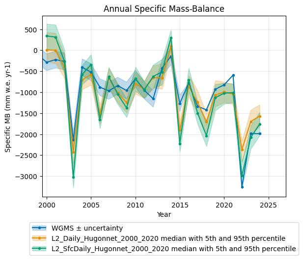
For the surface-tracking model, we see that the extreme year 2022 is captured much better. This improvement is likely related to the bucket-based snow-tracking system, which implicitly includes albedo feedbacks. In 2022, the glacier surface became snow-free very early, leading to a darker surface and therefore enhanced ablation.

However, the newly developed bucket system still requires further research and development before it can be considered operational.

A promising future direction is the assimilation of snowline observations. By including surface tracking, we are able to make use of this new type of EO data, in particular snowline altitudes derived from Sentinel-2. In the current implementation, these data are used only for validation, but future developments should make it possible to also include them directly in the assimilation pipeline.

The validation metrics of this first implementation are shown below:

validation_data_aut["Sentinel2"]

	MeanAbsD (m)	MeanD (m)	MedianD (m)	RMSD (m)	CORRCOEF
L1 Sentinel2 snowline 2015-07-04_2021-09-25
L2_SfcDaily_Hugonnet_2000_2020	109.1 (92.7, 133.0)	9.9 (-38.7, 53.6)	15.5 (-0.2, 15.5)	167.3 (138.8, 205.1)	0.80 (0.72, 0.87)

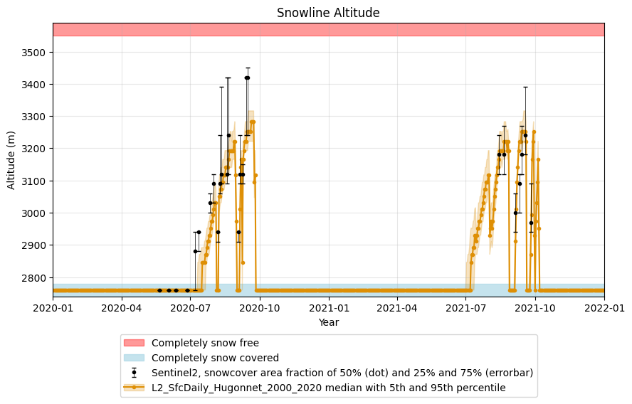
The modelled snowline evolution can also be visualised together with the observations:

validator_aut.get_validation_plot_for_layers(
    l2_name_list=l2_list_aut,
    obs_name="Sentinel2",
)
plt.show()

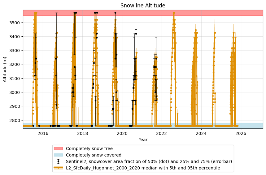
The plot is quite dense when shown over the full period. Therefore, you can use x_lim to zoom in on a specific period of interest:

validator_aut.get_validation_plot_for_layers(
    l2_name_list=l2_list_aut, obs_name="Sentinel2", x_lim=[2020, 2022]
)
plt.show()