


Creating DTC Glaciers EO-Native Data Cubes (L1)#
In this notebook, we focus on the creation of EO-native data cubes, referred to in the DTC Glaciers project as Level 1 (L1) data cubes.
L1 data cubes form the observational foundation of the DTC Glaciers workflow.
They consist exclusively of Earth Observation (EO) data and in-situ measurements, without the inclusion of model-derived or assimilated quantities. In line with the project design outlined in the proposal, L1 data cubes are generated for individual glaciers, providing a harmonised, analysis-ready representation of the available observations.
All variables within an L1 data cube are projected onto a common spatial grid, temporally aligned where applicable, and pre-processed to enable consistent use in subsequent stages of the DTC, including data assimilation, modelling, and validation workflows (L2 and beyond).
To illustrate the construction and content of L1 data cubes using different EO data sources, this notebook focuses on two contrasting case studies: the Brúarjökull outlet glacier of the Vatnajökull ice cap in Iceland, and Vernagtferner in the Ötztal Alps, Austria.
If required, install the DTCG API using the following command:
!pip install 'dtcg[jupyter] @ git+https://github.com/DTC-Glaciers/dtcg'
Run this command in a notebook cell.
# Imports
import dtcg.integration.oggm_bindings as oggm_bindings
import matplotlib.pyplot as plt
Downloading salem-sample-data...
rgi_id_ice = "RGI60-06.00377"  # Brúarjökull
rgi_id_aut = "RGI60-11.00719"  # Vernagtferner
Extract L1 data cubes from OGGM#
DTC Glaciers starts from glacier-domain datasets provided through the OGGM Shop, which aggregates products from multiple data providers and packages them into a data cube.
This step downloads the required pre-processed L1 data cubes from OGGM in the background and prepares the inputs needed to run the glacier model. This operation can take some time as it involves transferring data from the OGGM servers.
This download step is not required for end users: L1 and L2 data cubes are intended to be accessed directly as ready-to-use products (via GeoZarr). The workflow shown here illustrates the internal processes performed by the DTC Glaciers system to create and manage these data cubes.
dtcg_oggm_ice = oggm_bindings.BindingsOggmModel(rgi_id=rgi_id_ice)
dtcg_oggm_aut = oggm_bindings.BindingsOggmModel(rgi_id=rgi_id_aut)
Let’s have a look what OGGM supports out of the box:
dtcg_oggm_aut.datacube_l1
<xarray.Dataset> Size: 3MB
Dimensions:                  (y: 229, x: 254)
Coordinates:
  * y                        (y) float32 916B 5.199e+06 5.199e+06 ... 5.187e+06
  * x                        (x) float32 1kB 6.321e+05 6.322e+05 ... 6.45e+05
Data variables: (12/14)
    topo                     (y, x) float32 233kB 1.742e+03 ... 2.256e+03
    topo_smoothed            (y, x) float32 233kB 1.725e+03 ... 2.283e+03
    topo_valid_mask          (y, x) int8 58kB 1 1 1 1 1 1 1 1 ... 1 1 1 1 1 1 1
    glacier_mask             (y, x) int8 58kB 0 0 0 0 0 0 0 0 ... 0 0 0 0 0 0 0
    glacier_ext              (y, x) int8 58kB 0 0 0 0 0 0 0 0 ... 0 0 0 0 0 0 0
    consensus_ice_thickness  (y, x) float32 233kB nan nan nan ... nan nan nan
    ...                       ...
    itslive_vy               (y, x) float32 233kB -0.09633 -0.09943 ... 0.0
    millan_ice_thickness     (y, x) float32 233kB nan nan nan ... nan nan nan
    millan_v                 (y, x) float32 233kB nan nan nan ... nan nan nan
    millan_vx                (y, x) float32 233kB nan nan nan ... nan nan nan
    millan_vy                (y, x) float32 233kB nan nan nan ... nan nan nan
    hugonnet_dhdt            (y, x) float32 233kB 0.1893 0.1624 ... 0.001232
Attributes:
    author:              OGGM
    author_info:         Open Global Glacier Model
    pyproj_srs:          +proj=utm +zone=32 +datum=WGS84 +units=m +no_defs
    max_h_dem:           3737.275
    min_h_dem:           1701.9393
    max_h_glacier:       3574.82
    min_h_glacier:       2794.6978
    glacier_attributes:  {'rgi_id': 'RGI60-11.00719', 'glims_id': 'G010818E46...
RGI-ID: RGI60-11.00719- y: 229
- x: 254
- y(y)float325.199e+06 5.199e+06 ... 5.187e+06
- units :
- m
- long_name :
- y coordinate of projection
- standard_name :
- projection_y_coordinate
array([5.198700e+06, 5.198648e+06, 5.198598e+06, ..., 5.187174e+06, 5.187122e+06, 5.187072e+06], shape=(229,), dtype=float32) - x(x)float326.321e+05 6.322e+05 ... 6.45e+05
- units :
- m
- long_name :
- x coordinate of projection
- standard_name :
- projection_x_coordinate
array([632125.5, 632176.5, 632227.5, ..., 644926.5, 644977.5, 645028.5],
      shape=(254,), dtype=float32)
- topo(y, x)float321.742e+03 1.719e+03 ... 2.256e+03
- units :
- m
- long_name :
- DEM topography
array([[1742.0565, 1718.5181, 1704.2761, ..., 2634.5364, 2637.226 , 2649.449 ], [1740.664 , 1714.4333, 1704.7688, ..., 2638.1663, 2647.0886, 2669.9976], [1736.8108, 1715.1503, 1707.2252, ..., 2642.6921, 2663.412 , 2690.577 ], ..., [2751.1343, 2759.4119, 2786.9155, ..., 2333.323 , 2293.8684, 2260.5007], [2716.279 , 2725.114 , 2737.6365, ..., 2320.2432, 2284.971 , 2255.3079], [2691.5476, 2701.3706, 2716.6023, ..., 2306.4504, 2277.612 , 2256.4653]], shape=(229, 254), dtype=float32) - topo_smoothed(y, x)float321.725e+03 1.719e+03 ... 2.283e+03
- units :
- m
- long_name :
- DEM topography smoothed with radius: 3e+02 m
array([[1724.8086, 1719.3458, 1712.1177, ..., 2636.773 , 2646.762 , 2652.9497], [1724.4166, 1719.1144, 1712.0779, ..., 2641.2793, 2652.6218, 2659.8135], [1724.0541, 1718.9253, 1712.0941, ..., 2649.7158, 2663.504 , 2672.4287], ..., [2769.0166, 2785.2014, 2816.7178, ..., 2337.9739, 2310.3232, 2294.3115], [2743.747 , 2758.433 , 2787.9717, ..., 2328.795 , 2302.123 , 2286.7192], [2729.0059, 2742.7756, 2771.012 , ..., 2323.2456, 2297.5151, 2282.7017]], shape=(229, 254), dtype=float32) - topo_valid_mask(y, x)int81 1 1 1 1 1 1 1 ... 1 1 1 1 1 1 1 1
- units :
- -
- long_name :
- DEM validity mask according to geotiff input (1-0)
array([[1, 1, 1, ..., 1, 1, 1], [1, 1, 1, ..., 1, 1, 1], [1, 1, 1, ..., 1, 1, 1], ..., [1, 1, 1, ..., 1, 1, 1], [1, 1, 1, ..., 1, 1, 1], [1, 1, 1, ..., 1, 1, 1]], shape=(229, 254), dtype=int8) - glacier_mask(y, x)int80 0 0 0 0 0 0 0 ... 0 0 0 0 0 0 0 0
- units :
- -
- long_name :
- Glacier mask
array([[0, 0, 0, ..., 0, 0, 0], [0, 0, 0, ..., 0, 0, 0], [0, 0, 0, ..., 0, 0, 0], ..., [0, 0, 0, ..., 0, 0, 0], [0, 0, 0, ..., 0, 0, 0], [0, 0, 0, ..., 0, 0, 0]], shape=(229, 254), dtype=int8) - glacier_ext(y, x)int80 0 0 0 0 0 0 0 ... 0 0 0 0 0 0 0 0
- units :
- -
- long_name :
- Glacier external boundaries
array([[0, 0, 0, ..., 0, 0, 0], [0, 0, 0, ..., 0, 0, 0], [0, 0, 0, ..., 0, 0, 0], ..., [0, 0, 0, ..., 0, 0, 0], [0, 0, 0, ..., 0, 0, 0], [0, 0, 0, ..., 0, 0, 0]], shape=(229, 254), dtype=int8) - consensus_ice_thickness(y, x)float32nan nan nan nan ... nan nan nan nan
- units :
- m
- long_name :
- Ice thickness from the consensus estimate
- base_url :
- https://cluster.klima.uni-bremen.de/~fmaussion/icevol/composite/
array([[nan, nan, nan, ..., nan, nan, nan], [nan, nan, nan, ..., nan, nan, nan], [nan, nan, nan, ..., nan, nan, nan], ..., [nan, nan, nan, ..., nan, nan, nan], [nan, nan, nan, ..., nan, nan, nan], [nan, nan, nan, ..., nan, nan, nan]], shape=(229, 254), dtype=float32) - itslive_v(y, x)float320.2434 0.2606 ... 0.2455 0.2186
- units :
- m yr-1
- long_name :
- ITS LIVE velocity data
array([[0.24344647, 0.26063082, 0.25035125, ..., 0.3579173 , 0.33561128, 0.28883582], [0.215022 , 0.23906074, 0.23105459, ..., 0.23957004, 0.2915858 , 0.25415778], [0.2174102 , 0.22514711, 0.21218726, ..., 0.19214211, 0.23711233, 0.22129242], ..., [0.12075873, 0.10186059, 0.1240496 , ..., 0.38581932, 0.2984355 , 0.27908072], [0.12112405, 0.08944868, 0.11879443, ..., 0.3723072 , 0.2577669 , 0.24903257], [0.2777302 , 0.29464224, 0.36886322, ..., 0.32898155, 0.2455291 , 0.21862198]], shape=(229, 254), dtype=float32) - itslive_vx(y, x)float320.1682 0.183 ... -0.02476 -0.05019
- units :
- m yr-1
- long_name :
- ITS LIVE velocity data in x map direction
array([[ 0.16823728, 0.18299547, 0.21395968, ..., 0.14311485, 0.18160792, 0.16164705], [ 0.21357566, 0.23756774, 0.23035474, ..., 0.23543918, 0.28862417, 0.25171182], [ 0.2174102 , 0.22514711, 0.21218726, ..., 0.19214211, 0.23711233, 0.22129242], ..., [ 0.09323441, 0.05910604, 0.06591155, ..., -0.09302186, -0.16451906, -0.21805006], [ 0.06243233, 0.00519245, 0.00568864, ..., -0.12723948, -0.18808964, -0.2339943 ], [ 0.07564991, 0.05815558, 0.06371289, ..., -0.04651477, -0.02475613, -0.05019299]], shape=(229, 254), dtype=float32) - itslive_vy(y, x)float32-0.09633 -0.09943 ... -0.05135 0.0
- units :
- m yr-1
- long_name :
- ITS LIVE velocity data in y map direction
array([[-0.09632614, -0.09943351, -0.04660948, ..., -0.22293597, -0.16981854, -0.14407717], [-0.00185245, -0.0019122 , -0.00089635, ..., -0.00428728, -0.00326578, -0.00277075], [ 0. , 0. , 0. , ..., 0. , 0. , 0. ], ..., [ 0. , 0. , 0. , ..., -0.31767195, -0.16941534, -0.08806729], [-0.01928749, -0.02240353, -0.02785993, ..., -0.26921242, -0.06118476, 0. ], [-0.2160203 , -0.25092 , -0.3120319 , ..., -0.2259387 , -0.0513498 , 0. ]], shape=(229, 254), dtype=float32) - millan_ice_thickness(y, x)float32nan nan nan nan ... nan nan nan nan
- units :
- m
- long_name :
- Ice thickness from Millan et al. 2022
- data_source :
- RGI-11_2021July09
array([[nan, nan, nan, ..., nan, nan, nan], [nan, nan, nan, ..., nan, nan, nan], [nan, nan, nan, ..., nan, nan, nan], ..., [nan, nan, nan, ..., nan, nan, nan], [nan, nan, nan, ..., nan, nan, nan], [nan, nan, nan, ..., nan, nan, nan]], shape=(229, 254), dtype=float32) - millan_v(y, x)float32nan nan nan nan ... nan nan nan nan
- units :
- m
- long_name :
- Ice velocity from Millan et al. 2022
- data_source :
- RGI-11_2021July01
array([[nan, nan, nan, ..., nan, nan, nan], [nan, nan, nan, ..., nan, nan, nan], [nan, nan, nan, ..., nan, nan, nan], ..., [nan, nan, nan, ..., nan, nan, nan], [nan, nan, nan, ..., nan, nan, nan], [nan, nan, nan, ..., nan, nan, nan]], shape=(229, 254), dtype=float32) - millan_vx(y, x)float32nan nan nan nan ... nan nan nan nan
- units :
- m
- long_name :
- Ice velocity in map x direction from Millan et al. 2022
- data_source :
- RGI-11_2021July01
array([[nan, nan, nan, ..., nan, nan, nan], [nan, nan, nan, ..., nan, nan, nan], [nan, nan, nan, ..., nan, nan, nan], ..., [nan, nan, nan, ..., nan, nan, nan], [nan, nan, nan, ..., nan, nan, nan], [nan, nan, nan, ..., nan, nan, nan]], shape=(229, 254), dtype=float32) - millan_vy(y, x)float32nan nan nan nan ... nan nan nan nan
- units :
- m
- long_name :
- Ice velocity in map y direction from Millan et al. 2022
- data_source :
- RGI-11_2021July01
array([[nan, nan, nan, ..., nan, nan, nan], [nan, nan, nan, ..., nan, nan, nan], [nan, nan, nan, ..., nan, nan, nan], ..., [nan, nan, nan, ..., nan, nan, nan], [nan, nan, nan, ..., nan, nan, nan], [nan, nan, nan, ..., nan, nan, nan]], shape=(229, 254), dtype=float32) - hugonnet_dhdt(y, x)float320.1893 0.1624 ... 0.004438 0.001232
- units :
- m
- long_name :
- dhdt (2000-2020) from Hugonnet et al. 2021
- data_source :
- /home/data/download/cluster.klima.uni-bremen.de/~oggm/geodetic_ref_mb_maps/dhdt/N46E010_2000-01-01_2020-01-01_dhdt.tif
array([[ 1.8931952e-01,  1.6242915e-01,  1.4414129e-01, ...,
        -1.1726944e+00, -8.4028047e-01, -5.2263099e-01],
       [ 1.9792432e-01,  1.8828717e-01,  3.7784296e-01, ...,
        -1.0144438e+00, -6.3453114e-01, -3.5095587e-01],
       [ 2.0982631e-01,  2.2902362e-01,  6.1095959e-01, ...,
        -8.5337508e-01, -4.3152189e-01, -1.8335494e-01],
       ...,
       [-8.4933359e-03, -2.2932557e-02, -2.3965480e-02, ...,
        -7.7997725e-03, -7.1713943e-03, -5.7778261e-03],
       [-3.8133018e-02, -3.8725853e-02, -2.9151555e-02, ...,
        -9.8316406e-04,  4.3411115e-03,  3.5339131e-03],
       [-6.1521191e-02, -7.7394404e-02, -6.3811660e-02, ...,
        -1.6706563e-04,  4.4379705e-03,  1.2322172e-03]],
      shape=(229, 254), dtype=float32)
- author :
- OGGM
- author_info :
- Open Global Glacier Model
- pyproj_srs :
- +proj=utm +zone=32 +datum=WGS84 +units=m +no_defs
- max_h_dem :
- 3737.275
- min_h_dem :
- 1701.9393
- max_h_glacier :
- 3574.82
- min_h_glacier :
- 2794.6978
- glacier_attributes :
- {'rgi_id': 'RGI60-11.00719', 'glims_id': 'G010818E46876N', 'cenlon': 10.818, 'cenlat': 46.8762, 'rgi_region': '11', 'rgi_subregion': '11-01', 'rgi_version': '60', 'rgi_dem_source': 'COPDEM30', 'glacier_type': 'Glacier', 'terminus_type': 'Land-terminating', 'name': 'Vernagtferner', 'rgi_region_name': '11: Central Europe', 'rgi_subregion_name': '11-01: Alps ', 'rgi_date': 2003}
- RGI-ID :
- RGI60-11.00719
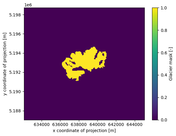
A central element of each data cube is the glacier outline which defines the spatial domain of the glacier.
The data cube domain is constructed by adding a buffer around this outline to ensure full coverage of the glacier and its immediate surroundings.
In the current implementation, we rely on Randolph Glacier Inventory (RGI) version 6 outlines.
This choice is driven by data availability and consistency, as most global glacier datasets currently in use have been processed based on RGI v6 outlines.
In future developments, the DTC Glaciers workflow is expected to transition to RGI version 7 as data products and community standards evolve.
Let’s have a look at the glacier outline used in this example:
glacier_mask_aut = dtcg_oggm_aut.datacube_l1.glacier_mask
glacier_mask_aut.plot();
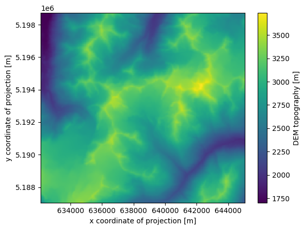
The data cubes already contain topographic information from the Copernicus DEM – Global and European Digital Elevation Model:
dtcg_oggm_aut.datacube_l1.topo.plot();
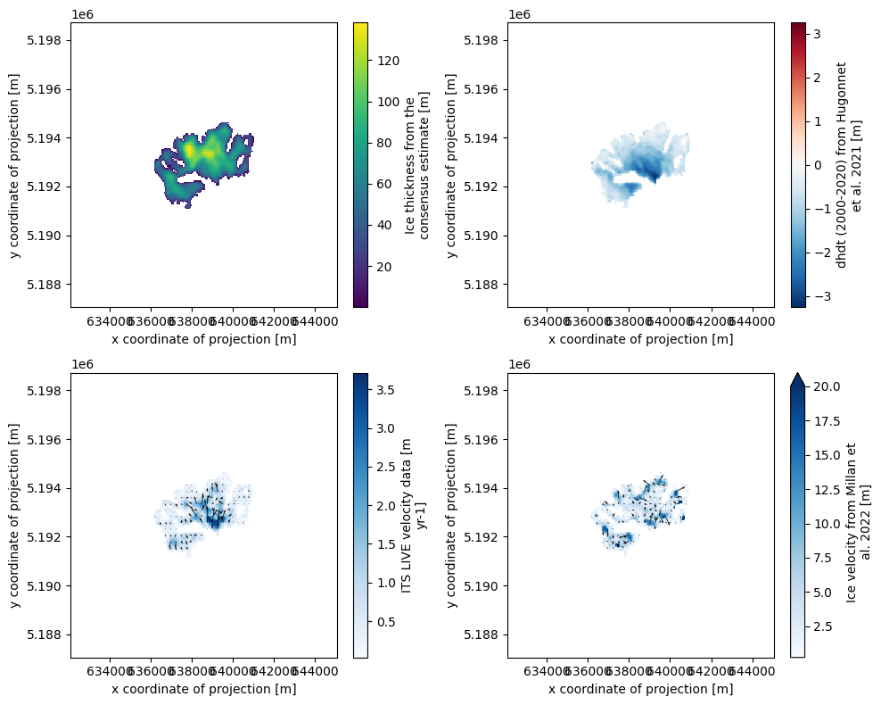
As well as:
Ice thickness data from Farinotti et al. (2019) (consensus estimate)
Elevation change data from Hugonnet et al. (2021)
Ice velocity data from ITS_LIVE
Ice velocity and ice thickness data from Millan et al. (2022)
Show code cell source
Hide code cell source
def plot_velocity(ax, ds, prefix, subsample=5, vmax=None):
    # subsample for vector clarity
    ds_q = ds.isel(x=slice(None, None, subsample), y=slice(None, None, subsample))

    # background scalar field
    ds[f"{prefix}_v"].plot(ax=ax, cmap="Blues", vmax=vmax)

    # vector overlay
    ax.quiver(
        ds_q["x"], ds_q["y"], ds_q[f"{prefix}_vx"], ds_q[f"{prefix}_vy"], color="black"
    )


fig, axs = plt.subplots(2, 2, figsize=(10, 8))

# Farinotti et al. (2019) ice thickness (consenus estimate)
dtcg_oggm_aut.datacube_l1.consensus_ice_thickness.plot(ax=axs[0, 0])

# Hugonnet et al. (2021) height change
dtcg_oggm_aut.datacube_l1.hugonnet_dhdt.where(glacier_mask_aut).plot(ax=axs[0, 1])

# ITS_LIVE ice velocity
plot_velocity(
    ax=axs[1, 0], ds=dtcg_oggm_aut.datacube_l1.where(glacier_mask_aut), prefix="itslive"
)

# Millan et al. (2022) ice velocity
plot_velocity(
    ax=axs[1, 1],
    ds=dtcg_oggm_aut.datacube_l1.where(glacier_mask_aut),
    prefix="millan",
    vmax=20,
)

plt.tight_layout()
plt.show()
Enhancing OGGM data cubes with new observations#
CryoTEMPO-EOLIS derived from CryoSat-2#
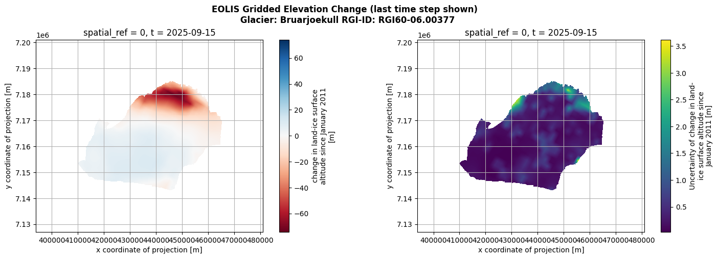
We developed a method to add four CryoTEMPO-EOLIS variables derived from CryoSat-2 observations to the L1 data cubes.
Variable |
Dims |
Description |
|---|---|---|
|
|
Time series of spatial maps of elevation change since January 2011. |
|
|
Uncertainty (σ) for the gridded elevation-change maps. |
|
|
Spatially aggregated 1D elevation-change series since January 2011. |
|
|
Uncertainty (σ) for the aggregated series. |
To use this on your own laptop, you need to register on the Specklia website and obtain an API key. You then need to provide this key to DTC Glaciers in the following way:
# import os
# os.environ["SPECKLIA_API_KEY"] = ENTER YOUR SPECKLIA API KEY HERE
You can add the data using add_data together with DatacubeCryotempoEolis. This step can take some time, as up-to-date data are downloaded from the CryoTEMPO-EOLIS server and reprojected to the L1 data cubes.
from dtcg.datacube.cryotempo_eolis import DatacubeCryotempoEolis

dtcg_oggm_ice.add_data(DatacubeCryotempoEolis)

dtcg_oggm_ice.datacube_l1
<xarray.Dataset> Size: 464MB
Dimensions:                                  (y: 370, x: 436, t: 177)
Coordinates:
  * y                                        (y) float32 1kB 7.201e+06 ... 7....
  * x                                        (x) float32 2kB 3.94e+05 ... 4.8...
  * t                                        (t) int64 1kB 1295049600 ... 175...
    spatial_ref                              int64 8B 0
Data variables: (12/18)
    topo                                     (y, x) float32 645kB 1.147e+03 ....
    topo_smoothed                            (y, x) float32 645kB 1.151e+03 ....
    topo_valid_mask                          (y, x) int8 161kB 1 1 1 1 ... 1 1 1
    glacier_mask                             (y, x) int8 161kB 0 0 0 0 ... 0 0 0
    glacier_ext                              (y, x) int8 161kB 0 0 0 0 ... 0 0 0
    consensus_ice_thickness                  (y, x) float32 645kB nan ... nan
    ...                                       ...
    millan_vy                                (y, x) float32 645kB nan ... nan
    hugonnet_dhdt                            (y, x) float32 645kB nan ... -0....
    eolis_gridded_elevation_change           (t, y, x) float64 228MB nan ... nan
    eolis_gridded_elevation_change_sigma     (t, y, x) float64 228MB nan ... nan
    eolis_elevation_change_timeseries        (t) float64 1kB 0.0 ... -5.208
    eolis_elevation_change_sigma_timeseries  (t) float64 1kB 0.0 ... 0.3651
Attributes:
    author:              OGGM
    author_info:         Open Global Glacier Model
    pyproj_srs:          +proj=utm +zone=28 +datum=WGS84 +units=m +no_defs
    max_h_dem:           1901.579
    min_h_dem:           -0.24698931
    max_h_glacier:       1875.962
    min_h_glacier:       623.5142
    glacier_attributes:  {'rgi_id': 'RGI60-06.00377', 'glims_id': 'G343733E64...
RGI-ID: RGI60-06.00377- y: 370
- x: 436
- t: 177
- y(y)float327.201e+06 7.201e+06 ... 7.127e+06
- units :
- m
- long_name :
- y coordinate of projection
- standard_name :
- projection_y_coordinate
array([7.200982e+06, 7.200782e+06, 7.200582e+06, ..., 7.127582e+06, 7.127382e+06, 7.127182e+06], shape=(370,), dtype=float32) - x(x)float323.94e+05 3.942e+05 ... 4.81e+05
- units :
- m
- long_name :
- x coordinate of projection
- standard_name :
- projection_x_coordinate
array([393962.1, 394162.1, 394362.1, ..., 480562.1, 480762.1, 480962.1], shape=(436,), dtype=float32) - t(t)int641295049600 ... 1757894400
- standard_name :
- time
- long_name :
- time since the unix epoch
- units :
- seconds since 1970-01-01 00:00:00
array([1295049600, 1297728000, 1300147200, 1302825600, 1305417600, 1308096000, 1310688000, 1313366400, 1316044800, 1318636800, 1321315200, 1323907200, 1326585600, 1329264000, 1331769600, 1334448000, 1337040000, 1339718400, 1342310400, 1344988800, 1347667200, 1350259200, 1352937600, 1355529600, 1358208000, 1360886400, 1363305600, 1365984000, 1368576000, 1371254400, 1373846400, 1376524800, 1379203200, 1381795200, 1384473600, 1387065600, 1389744000, 1392422400, 1394841600, 1397520000, 1400112000, 1402790400, 1405382400, 1408060800, 1410739200, 1413331200, 1416009600, 1418601600, 1421280000, 1423958400, 1426377600, 1429056000, 1431648000, 1434326400, 1436918400, 1439596800, 1442275200, 1444867200, 1447545600, 1450137600, 1452816000, 1455494400, 1458000000, 1460678400, 1463270400, 1465948800, 1468540800, 1471219200, 1473897600, 1476489600, 1479168000, 1481760000, 1484438400, 1487116800, 1489536000, 1492214400, 1494806400, 1497484800, 1500076800, 1502755200, 1505433600, 1508025600, 1510704000, 1513296000, 1515974400, 1518652800, 1521072000, 1523750400, 1526342400, 1529020800, 1531612800, 1534291200, 1536969600, 1539561600, 1542240000, 1544832000, 1547510400, 1550188800, 1552608000, 1555286400, 1557878400, 1560556800, 1563148800, 1565827200, 1568505600, 1571097600, 1573776000, 1576368000, 1579046400, 1581724800, 1584230400, 1586908800, 1589500800, 1592179200, 1594771200, 1597449600, 1600128000, 1602720000, 1605398400, 1607990400, 1610668800, 1613347200, 1615766400, 1618444800, 1621036800, 1623715200, 1626307200, 1628985600, 1631664000, 1634256000, 1636934400, 1639526400, 1642204800, 1644883200, 1647302400, 1649980800, 1652572800, 1655251200, 1657843200, 1660521600, 1663200000, 1665792000, 1668470400, 1671062400, 1673740800, 1676419200, 1678838400, 1681516800, 1684108800, 1686787200, 1689379200, 1692057600, 1694736000, 1697328000, 1700006400, 1702598400, 1705276800, 1707955200, 1710460800, 1713139200, 1715731200, 1718409600, 1721001600, 1723680000, 1726358400, 1728950400, 1731628800, 1734220800, 1736899200, 1739577600, 1741996800, 1744675200, 1747267200, 1749945600, 1752537600, 1755216000, 1757894400]) - spatial_ref()int640
- crs_wkt :
- PROJCS["unknown",GEOGCS["unknown",DATUM["WGS_1984",SPHEROID["WGS 84",6378137,298.257223563,AUTHORITY["EPSG","7030"]],AUTHORITY["EPSG","6326"]],PRIMEM["Greenwich",0,AUTHORITY["EPSG","8901"]],UNIT["degree",0.0174532925199433,AUTHORITY["EPSG","9122"]]],PROJECTION["Transverse_Mercator"],PARAMETER["latitude_of_origin",0],PARAMETER["central_meridian",-15],PARAMETER["scale_factor",0.9996],PARAMETER["false_easting",500000],PARAMETER["false_northing",0],UNIT["metre",1,AUTHORITY["EPSG","9001"]],AXIS["Easting",EAST],AXIS["Northing",NORTH]]
- semi_major_axis :
- 6378137.0
- semi_minor_axis :
- 6356752.314245179
- inverse_flattening :
- 298.257223563
- reference_ellipsoid_name :
- WGS 84
- longitude_of_prime_meridian :
- 0.0
- prime_meridian_name :
- Greenwich
- geographic_crs_name :
- unknown
- horizontal_datum_name :
- World Geodetic System 1984
- projected_crs_name :
- unknown
- grid_mapping_name :
- transverse_mercator
- latitude_of_projection_origin :
- 0.0
- longitude_of_central_meridian :
- -15.0
- false_easting :
- 500000.0
- false_northing :
- 0.0
- scale_factor_at_central_meridian :
- 0.9996
- spatial_ref :
- PROJCS["unknown",GEOGCS["unknown",DATUM["WGS_1984",SPHEROID["WGS 84",6378137,298.257223563,AUTHORITY["EPSG","7030"]],AUTHORITY["EPSG","6326"]],PRIMEM["Greenwich",0,AUTHORITY["EPSG","8901"]],UNIT["degree",0.0174532925199433,AUTHORITY["EPSG","9122"]]],PROJECTION["Transverse_Mercator"],PARAMETER["latitude_of_origin",0],PARAMETER["central_meridian",-15],PARAMETER["scale_factor",0.9996],PARAMETER["false_easting",500000],PARAMETER["false_northing",0],UNIT["metre",1,AUTHORITY["EPSG","9001"]],AXIS["Easting",EAST],AXIS["Northing",NORTH]]
array(0)
- topo(y, x)float321.147e+03 1.141e+03 ... 0.0 0.0
- units :
- m
- long_name :
- DEM topography
array([[1.1469581e+03, 1.1407299e+03, 1.1381298e+03, ..., 6.6475842e+02, 6.5947559e+02, 6.5525848e+02], [1.1705750e+03, 1.1692976e+03, 1.1588870e+03, ..., 6.6196667e+02, 6.5631232e+02, 6.5455737e+02], [1.2064128e+03, 1.2036810e+03, 1.1891963e+03, ..., 6.5896118e+02, 6.5506055e+02, 6.5444885e+02], ..., [8.8076691e+02, 8.6122577e+02, 8.8352625e+02, ..., 2.6724836e-01, 1.7347394e-01, 1.9891816e-01], [8.6362506e+02, 8.5418347e+02, 8.8737177e+02, ..., 0.0000000e+00, 0.0000000e+00, 0.0000000e+00], [8.4890240e+02, 8.5093469e+02, 8.8949481e+02, ..., 0.0000000e+00, 0.0000000e+00, 0.0000000e+00]], shape=(370, 436), dtype=float32) - topo_smoothed(y, x)float321.151e+03 1.147e+03 ... 0.0002844
- units :
- m
- long_name :
- DEM topography smoothed with radius: 3e+02 m
array([[1.1508660e+03, 1.1469803e+03, 1.1412454e+03, ..., 6.6404663e+02, 6.5915826e+02, 6.5589307e+02], [1.1726067e+03, 1.1690500e+03, 1.1603943e+03, ..., 6.6184216e+02, 6.5738916e+02, 6.5511414e+02], [1.2069194e+03, 1.2019698e+03, 1.1898363e+03, ..., 6.5961139e+02, 6.5609778e+02, 6.5490656e+02], ..., [8.7737811e+02, 8.7143109e+02, 8.8398639e+02, ..., 1.9621927e-01, 1.4236444e-01, 1.5236741e-01], [8.6219836e+02, 8.6371283e+02, 8.8232770e+02, ..., 1.7820445e-01, 4.1718520e-02, 4.0628150e-02], [8.5193823e+02, 8.5963940e+02, 8.8198364e+02, ..., 1.4999704e-01, 9.4814815e-05, 2.8444445e-04]], shape=(370, 436), dtype=float32) - topo_valid_mask(y, x)int81 1 1 1 1 1 1 1 ... 1 1 1 1 1 1 1 1
- units :
- -
- long_name :
- DEM validity mask according to geotiff input (1-0)
array([[1, 1, 1, ..., 1, 1, 1], [1, 1, 1, ..., 1, 1, 1], [1, 1, 1, ..., 1, 1, 1], ..., [1, 1, 1, ..., 1, 1, 1], [1, 1, 1, ..., 1, 1, 1], [1, 1, 1, ..., 1, 1, 1]], shape=(370, 436), dtype=int8) - glacier_mask(y, x)int80 0 0 0 0 0 0 0 ... 0 0 0 0 0 0 0 0
- units :
- -
- long_name :
- Glacier mask
array([[0, 0, 0, ..., 0, 0, 0], [0, 0, 0, ..., 0, 0, 0], [0, 0, 0, ..., 0, 0, 0], ..., [0, 0, 0, ..., 0, 0, 0], [0, 0, 0, ..., 0, 0, 0], [0, 0, 0, ..., 0, 0, 0]], shape=(370, 436), dtype=int8) - glacier_ext(y, x)int80 0 0 0 0 0 0 0 ... 0 0 0 0 0 0 0 0
- units :
- -
- long_name :
- Glacier external boundaries
array([[0, 0, 0, ..., 0, 0, 0], [0, 0, 0, ..., 0, 0, 0], [0, 0, 0, ..., 0, 0, 0], ..., [0, 0, 0, ..., 0, 0, 0], [0, 0, 0, ..., 0, 0, 0], [0, 0, 0, ..., 0, 0, 0]], shape=(370, 436), dtype=int8) - consensus_ice_thickness(y, x)float32nan nan nan nan ... nan nan nan nan
- units :
- m
- long_name :
- Ice thickness from the consensus estimate
- base_url :
- https://cluster.klima.uni-bremen.de/~fmaussion/icevol/composite/
array([[nan, nan, nan, ..., nan, nan, nan], [nan, nan, nan, ..., nan, nan, nan], [nan, nan, nan, ..., nan, nan, nan], ..., [nan, nan, nan, ..., nan, nan, nan], [nan, nan, nan, ..., nan, nan, nan], [nan, nan, nan, ..., nan, nan, nan]], shape=(370, 436), dtype=float32) - itslive_v(y, x)float320.2549 0.316 0.104 ... nan nan nan
- units :
- m yr-1
- long_name :
- ITS LIVE velocity data
array([[0.2548638 , 0.3160016 , 0.1039561 , ..., 0.9141536 , 0.8403372 , 0.69694364], [0.27767682, 0.24819988, 0.28476351, ..., 2.0485506 , 1.150246 , 0.50836325], [0.24675122, 0.27259168, 0.39868486, ..., 1.292929 , 0.61550474, 0.7452541 ], ..., [2.608234 , 1.8436593 , 2.698295 , ..., 0.37593848, 0.3458429 , 0.17436156], [1.7304813 , 1.645862 , 2.7974434 , ..., 0.331727 , 0.3038549 , nan], [2.200289 , 1.1182725 , 1.0266634 , ..., nan, nan, nan]], shape=(370, 436), dtype=float32) - itslive_vx(y, x)float320.09866 -0.03163 ... nan nan
- units :
- m yr-1
- long_name :
- ITS LIVE velocity data in x map direction
array([[ 0.09866323, -0.03163351, 0.01193277, ..., 0.43653226, 0.27403608, 0.6505354 ], [ 0.13080858, -0.05709021, -0.10543129, ..., 1.1964303 , 0.8653776 , 0.37876108], [-0.00792862, -0.09918541, 0.02574821, ..., 1.2704426 , 0.5189546 , 0.54376847], ..., [ 2.0647523 , 1.4015841 , 1.7450721 , ..., 0.1196125 , 0.07965311, 0.15799367], [ 0.7335261 , 0.9962476 , 1.6772281 , ..., 0.22557321, -0.0558848 , nan], [-0.40105644, 0.01473092, 0.09578909, ..., nan, nan, nan]], shape=(370, 436), dtype=float32) - itslive_vy(y, x)float320.2295 0.2614 -0.03591 ... nan nan
- units :
- m yr-1
- long_name :
- ITS LIVE velocity data in y map direction
array([[ 0.22947061, 0.26136097, -0.03591328, ..., -0.7614408 , -0.6316691 , 0.22846651], [ 0.24175306, 0.20272225, 0.14519516, ..., -1.484786 , -0.49687907, 0.33401275], [ 0.19546762, 0.20999992, 0.34258327, ..., -0.16592711, -0.03522476, 0.5024078 ], ..., [-1.588773 , -1.1954372 , -2.0550158 , ..., 0.34108493, 0.2978283 , -0.05139158], [-1.5430518 , -1.2969788 , -2.225027 , ..., 0.23560417, 0.1571845 , nan], [-2.065821 , -1.0968022 , -0.9228701 , ..., nan, nan, nan]], shape=(370, 436), dtype=float32) - millan_ice_thickness(y, x)float32nan nan nan nan ... nan nan nan nan
- units :
- m
- long_name :
- Ice thickness from Millan et al. 2022
- data_source :
- RGI-6_2021July09
array([[ nan, nan, nan, ..., nan, nan, nan], [ nan, nan, nan, ..., nan, nan, nan], [ nan, nan, nan, ..., nan, nan, nan], ..., [136.74094 , 105.654655, 107.06039 , ..., nan, nan, nan], [134.29288 , 80.722015, 122.45349 , ..., nan, nan, nan], [119.59741 , 124.96882 , 146.8433 , ..., nan, nan, nan]], shape=(370, 436), dtype=float32) - millan_v(y, x)float32nan nan nan nan ... nan nan nan nan
- units :
- m
- long_name :
- Ice velocity from Millan et al. 2022
- data_source :
- RGI-6_2021July01
array([[ nan, nan, nan, ..., nan, nan, nan], [ nan, nan, nan, ..., nan, nan, nan], [ nan, nan, nan, ..., nan, nan, nan], ..., [6.5736976 , 2.5098248 , 2.6613255 , ..., nan, nan, nan], [5.3003016 , 0.76216197, 3.846327 , ..., nan, nan, nan], [2.8178496 , 3.446664 , 6.557965 , ..., nan, nan, nan]], shape=(370, 436), dtype=float32) - millan_vx(y, x)float32nan nan nan nan ... nan nan nan nan
- units :
- m
- long_name :
- Ice velocity in map x direction from Millan et al. 2022
- data_source :
- RGI-6_2021July01
array([[ nan, nan, nan, ..., nan, nan, nan], [ nan, nan, nan, ..., nan, nan, nan], [ nan, nan, nan, ..., nan, nan, nan], ..., [ 5.7376456, 2.500143 , -0.41456 , ..., nan, nan, nan], [ 4.579548 , 0.730334 , -2.2977247, ..., nan, nan, nan], [ 2.8041666, -1.5834544, -4.262885 , ..., nan, nan, nan]], shape=(370, 436), dtype=float32) - millan_vy(y, x)float32nan nan nan nan ... nan nan nan nan
- units :
- m
- long_name :
- Ice velocity in map y direction from Millan et al. 2022
- data_source :
- RGI-6_2021July01
array([[ nan, nan, nan, ..., nan, nan, nan], [ nan, nan, nan, ..., nan, nan, nan], [ nan, nan, nan, ..., nan, nan, nan], ..., [-3.2082582 , -0.22023903, 2.6288388 , ..., nan, nan, nan], [-2.6685088 , 0.21795207, 3.0845897 , ..., nan, nan, nan], [ 0.2773556 , 3.0613992 , 4.9834437 , ..., nan, nan, nan]], shape=(370, 436), dtype=float32) - hugonnet_dhdt(y, x)float32nan nan nan ... -0.04221 -0.09642
- units :
- m
- long_name :
- dhdt (2000-2020) from Hugonnet et al. 2021
- data_source :
- /home/data/download/cluster.klima.uni-bremen.de/~oggm/geodetic_ref_mb_maps/dhdt/N64W017_2000-01-01_2020-01-01_dhdt.tif /home/data/download/cluster.klima.uni-bremen.de/~oggm/geodetic_ref_mb_maps/dhdt/N64W016_2000-01-01_2020-01-01_dhdt.tif
array([[ nan, nan, nan, ..., nan, nan, nan], [ nan, nan, nan, ..., nan, nan, nan], [ nan, nan, nan, ..., nan, nan, nan], ..., [ nan, nan, nan, ..., 0.01044447, -0.03536606, -0.00273148], [ nan, nan, nan, ..., -0.02919118, -0.0053511 , -0.01536089], [ nan, nan, nan, ..., -0.05867972, -0.04220677, -0.09641694]], shape=(370, 436), dtype=float32) - eolis_gridded_elevation_change(t, y, x)float64nan nan nan nan ... nan nan nan nan
- units :
- m
- ancillary_variables :
- elevation_change_sigma, interpolation_binary_mask
- comment :
- Elevation change since January 2011.
- institution :
- Earthwave/The University of Edinburgh/ESA
- long_name :
- change in land-ice surface altitude since January 2011
- references :
- EOLIS elevation data generated using swath processing of CryoSat-2 data (Jakob & Gourmelen, 2023) and provided by the ESA CryoTEMPO project (https://cryotempo-eolis.org/). Jakob, L., and Gourmelen, N., (2023). Glacier Mass Loss Between 2010 and 2020 Dominated by Atmospheric Forcing. Geophysical Research Letters 50(8), 1-10. doi:10.1029/2023GL102954
- source :
- CryoTEMPO-EOLIS gridded product; gaps filled with GPR. Observed values retained; only missing cells interpolated.
- standard_name :
- change_over_time_in_land_ice_surface_altitude
array([[[nan, nan, nan, ..., nan, nan, nan], [nan, nan, nan, ..., nan, nan, nan], [nan, nan, nan, ..., nan, nan, nan], ..., [nan, nan, nan, ..., nan, nan, nan], [nan, nan, nan, ..., nan, nan, nan], [nan, nan, nan, ..., nan, nan, nan]], [[nan, nan, nan, ..., nan, nan, nan], [nan, nan, nan, ..., nan, nan, nan], [nan, nan, nan, ..., nan, nan, nan], ..., [nan, nan, nan, ..., nan, nan, nan], [nan, nan, nan, ..., nan, nan, nan], [nan, nan, nan, ..., nan, nan, nan]], [[nan, nan, nan, ..., nan, nan, nan], [nan, nan, nan, ..., nan, nan, nan], [nan, nan, nan, ..., nan, nan, nan], ..., ... ..., [nan, nan, nan, ..., nan, nan, nan], [nan, nan, nan, ..., nan, nan, nan], [nan, nan, nan, ..., nan, nan, nan]], [[nan, nan, nan, ..., nan, nan, nan], [nan, nan, nan, ..., nan, nan, nan], [nan, nan, nan, ..., nan, nan, nan], ..., [nan, nan, nan, ..., nan, nan, nan], [nan, nan, nan, ..., nan, nan, nan], [nan, nan, nan, ..., nan, nan, nan]], [[nan, nan, nan, ..., nan, nan, nan], [nan, nan, nan, ..., nan, nan, nan], [nan, nan, nan, ..., nan, nan, nan], ..., [nan, nan, nan, ..., nan, nan, nan], [nan, nan, nan, ..., nan, nan, nan], [nan, nan, nan, ..., nan, nan, nan]]], shape=(177, 370, 436)) - eolis_gridded_elevation_change_sigma(t, y, x)float64nan nan nan nan ... nan nan nan nan
- units :
- m
- comment :
- Mixture of observational and GPR uncertainties, aligned to elevation_change.
- institution :
- Earthwave/The University of Edinburgh/ESA
- long_name :
- Uncertainty of change in land-ice surface altitude since January 2011
- references :
- EOLIS elevation data generated using swath processing of CryoSat-2 data (Jakob & Gourmelen, 2023) and provided by the ESA CryoTEMPO project (https://cryotempo-eolis.org/). Jakob, L., and Gourmelen, N., (2023). Glacier Mass Loss Between 2010 and 2020 Dominated by Atmospheric Forcing. Geophysical Research Letters 50(8), 1-10. doi:10.1029/2023GL102954
- source :
- Observed cells: CryoTEMPO-EOLIS uncertainties; interpolated cells: GPR predictive standard deviation.
- standard_name :
- change_over_time_in_land_ice_surface_altitude_standard_error
array([[[nan, nan, nan, ..., nan, nan, nan], [nan, nan, nan, ..., nan, nan, nan], [nan, nan, nan, ..., nan, nan, nan], ..., [nan, nan, nan, ..., nan, nan, nan], [nan, nan, nan, ..., nan, nan, nan], [nan, nan, nan, ..., nan, nan, nan]], [[nan, nan, nan, ..., nan, nan, nan], [nan, nan, nan, ..., nan, nan, nan], [nan, nan, nan, ..., nan, nan, nan], ..., [nan, nan, nan, ..., nan, nan, nan], [nan, nan, nan, ..., nan, nan, nan], [nan, nan, nan, ..., nan, nan, nan]], [[nan, nan, nan, ..., nan, nan, nan], [nan, nan, nan, ..., nan, nan, nan], [nan, nan, nan, ..., nan, nan, nan], ..., ... ..., [nan, nan, nan, ..., nan, nan, nan], [nan, nan, nan, ..., nan, nan, nan], [nan, nan, nan, ..., nan, nan, nan]], [[nan, nan, nan, ..., nan, nan, nan], [nan, nan, nan, ..., nan, nan, nan], [nan, nan, nan, ..., nan, nan, nan], ..., [nan, nan, nan, ..., nan, nan, nan], [nan, nan, nan, ..., nan, nan, nan], [nan, nan, nan, ..., nan, nan, nan]], [[nan, nan, nan, ..., nan, nan, nan], [nan, nan, nan, ..., nan, nan, nan], [nan, nan, nan, ..., nan, nan, nan], ..., [nan, nan, nan, ..., nan, nan, nan], [nan, nan, nan, ..., nan, nan, nan], [nan, nan, nan, ..., nan, nan, nan]]], shape=(177, 370, 436)) - eolis_elevation_change_timeseries(t)float640.0 0.4243 0.6179 ... -4.711 -5.208
- units :
- m
- ancillary_variables :
- eolis_elevation_change_sigma_timeseries
- comment :
- Computed from eolis_gridded_elevation_change. Elevation change since January 2011.
- institution :
- Earthwave/The University of Edinburgh/ESA
- long_name :
- change in land-ice surface altitude since January 2011
- references :
- EOLIS elevation data generated using swath processing of CryoSat-2 data (Jakob & Gourmelen, 2023) and provided by the ESA CryoTEMPO project (https://cryotempo-eolis.org/). Jakob, L., and Gourmelen, N., (2023). Glacier Mass Loss Between 2010 and 2020 Dominated by Atmospheric Forcing. Geophysical Research Letters 50(8), 1-10. doi:10.1029/2023GL102954
- source :
- CryoTEMPO-EOLIS gridded product; gaps filled with GPR. Observed values retained; only missing cells interpolated. Values represent glacier-wide mean elevation change, computed as the average of all valid grid cells (eolis_gridded_elevation_change) within the glacier mask.
- standard_name :
- change_over_time_in_land_ice_surface_altitude
array([ 0. , 0.42427715, 0.61787093, 0.79810586, 1.280484 , 1.65063014, 1.25216719, 0.14517839, -0.26150756, 0.03465799, 0.18777452, 0.2825392 , 0.31601209, 0.61030712, 1.08330959, 1.38053348, 1.360335 , 0.81153161, 0.18647484, -0.90209714, -1.46476251, -1.38025417, -1.08356517, -0.68222865, -0.22072183, 0.20963449, 0.4247909 , 0.37902378, 0.52773512, 0.32930434, -0.04009857, -1.19168916, -1.86307345, -1.88363253, -1.61707992, -1.34493563, -0.68005601, -0.06053428, 0.56657534, 0.76932105, 0.76616969, 0.44578643, -0.2541758 , -1.0893542 , -1.72861303, -1.70205495, -1.46251139, -1.1740918 , -0.88142969, -0.4547719 , -0.19332528, 0.01777152, 0.37037219, 0.72440244, 0.9029684 , 0.53122977, 0.05373315, -0.09301531, -0.1006654 , 0.06160301, 0.37005815, 0.83511389, 1.05159569, 1.28467112, 1.22382304, 1.14595591, 0.72963683, 0.1342616 , -0.5267253 , -0.68991262, -0.59772689, -0.40091844, -0.00731276, 0.45438711, 0.71553531, 0.95760455, 0.98035534, 0.90323193, 0.47579904, -0.21159103, -0.6934465 , -0.86136664, -0.89172437, -0.74678315, -0.31624511, 0.44652964, 0.83568759, 1.00216288, 0.98801802, 0.56638768, -0.21793997, -1.06160015, -1.32324369, -1.25197038, -0.92725956, -0.35763243, -0.11423192, 0.24763977, 0.63762506, 0.90857783, 0.61447516, -0.19921605, -1.07834618, -1.58448492, -1.76824464, -1.61346977, -1.47675418, -1.45468174, -1.19554447, -0.67519853, -0.29239861, 0.1006228 , -0.2072922 , -0.52358005, -1.20403128, -1.63565066, -2.08449769, -1.96817809, -1.9438345 , -1.43758794, -0.90815625, -0.35156128, -0.18463644, -0.05475687, -0.42427706, -0.9336288 , -1.55081401, -1.93471631, -2.54339691, -2.50226553, -2.53377705, -2.20957043, -2.07782054, -1.34420034, -1.09471477, -0.83183854, -0.7112665 , -0.99860041, -1.97719295, -2.55554598, -3.01992078, -2.69465982, -2.29544096, -1.98962091, -1.83057925, -1.54351837, -1.27888495, -0.89388655, -0.8745322 , -1.55630842, -2.65288091, -3.42853527, -3.98250467, -3.88129031, -4.02235728, -4.02801754, -3.72001533, -2.81772406, -2.57666514, -2.02418583, -2.02704592, -2.13149104, -3.16910302, -3.89534196, -4.37395442, -4.00411726, -4.13078748, -4.12287309, -3.90649851, -2.77201609, -2.05849591, -1.45056392, -1.71155506, -2.80037208, -4.0426447 , -4.71082568, -5.20822695]) - eolis_elevation_change_sigma_timeseries(t)float640.0 0.175 0.2359 ... 0.4634 0.3651
- units :
- m
- comment :
- Uncertainty propagated using a static 20 km spatial correlation length.
- institution :
- Earthwave/The University of Edinburgh/ESA
- long_name :
- Uncertainty of change in land-ice surface altitude since January 2011
- references :
- EOLIS elevation data generated using swath processing of CryoSat-2 data (Jakob & Gourmelen, 2023) and provided by the ESA CryoTEMPO project (https://cryotempo-eolis.org/). Jakob, L., and Gourmelen, N., (2023). Glacier Mass Loss Between 2010 and 2020 Dominated by Atmospheric Forcing. Geophysical Research Letters 50(8), 1-10. doi:10.1029/2023GL102954
- source :
- Observed cells: CryoTEMPO-EOLIS uncertainties; interpolated cells: GPR predictive standard deviation.Values represent propagated 1-sigma uncertainty of the glacier-wide mean, estimated from pixel-level uncertainties (eolis_gridded_elevation_change_sigma) using a spatial correlation model.
- standard_name :
- change_over_time_in_land_ice_surface_altitude_standard_error
- ancillary_variables :
- eolis_elevation_change_timeseries
array([0.        , 0.17498644, 0.23587579, 0.27230233, 0.25393823,
       0.25250553, 0.25670014, 0.24583876, 0.25159554, 0.25158392,
       0.25954046, 0.27353302, 0.27911986, 0.26998583, 0.29733875,
       0.40275033, 0.38123772, 0.27709962, 0.25826464, 0.27180151,
       0.26642008, 0.24772041, 0.25743374, 0.26908264, 0.27000194,
       0.28132047, 0.28618076, 0.2865384 , 0.30831451, 0.30877342,
       0.33145589, 0.25671396, 0.2447425 , 0.23420756, 0.26300223,
       0.33203067, 0.28429863, 0.28775724, 0.28322147, 0.33686582,
       0.34191558, 0.31441558, 0.24646535, 0.22936147, 0.23924597,
       0.2318304 , 0.25923973, 0.26804468, 0.26362977, 0.26302192,
       0.26399688, 0.35589051, 0.27712069, 0.28827616, 0.2859172 ,
       0.27029291, 0.24166285, 0.24859597, 0.30308305, 0.3515353 ,
       0.34640202, 0.3476224 , 0.33845384, 0.27575438, 0.27398536,
       0.26285927, 0.26660781, 0.25099435, 0.25508115, 0.25255473,
       0.24613484, 0.25796654, 0.25710347, 0.27142332, 0.24998987,
       0.31159682, 0.31029688, 0.2666854 , 0.26698807, 0.40018539,
       0.32039069, 0.27015262, 0.25245095, 0.28370898, 0.27712561,
       0.27031601, 0.27099898, 0.28258492, 0.29463599, 0.28318251,
       0.27365439, 0.30221946, 0.3142726 , 0.32893922, 0.33924956,
       0.31226633, 0.29770702, 0.28546843, 0.29420755, 0.31831126,
       0.28322658, 0.26532804, 0.25952487, 0.32566487, 0.32285851,
       0.37745027, 0.29977039, 0.46081057, 0.4866649 , 0.38094799,
       0.33283751, 0.31030085, 0.29485965, 0.31818766, 0.52537822,
       0.49153544, 0.37668961, 0.34456504, 0.38543129, 0.47037753,
       0.38024137, 0.31373979, 0.33552865, 0.90922764, 0.47521868,
       0.37989477, 0.39929585, 0.46651517, 0.70229366, 0.32522742,
       0.38270928, 0.44163541, 0.43843069, 0.33278047, 0.38415001,
       0.47077059, 0.86671346, 0.96278246, 0.53766543, 0.355081  ,
       0.42967192, 0.48775444, 0.46031838, 0.38653529, 0.39095639,
       0.90791935, 0.41550614, 0.42089979, 0.59767216, 0.79155722,
       0.70639985, 0.83545728, 0.75225982, 0.73184422, 0.39435281,
       0.37938765, 0.45570493, 1.00208709, 0.46309727, 0.4424133 ,
       0.43716356, 0.57354715, 0.9403413 , 0.39690144, 0.3419071 ,
       0.76315208, 0.39209244, 0.3641208 , 0.50816081, 0.64636323,
       0.53087383, 0.38396328, 0.41519856, 0.4892835 , 0.50840281,
       0.46341253, 0.36511708])
- author :
- OGGM
- author_info :
- Open Global Glacier Model
- pyproj_srs :
- +proj=utm +zone=28 +datum=WGS84 +units=m +no_defs
- max_h_dem :
- 1901.579
- min_h_dem :
- -0.24698931
- max_h_glacier :
- 1875.962
- min_h_glacier :
- 623.5142
- glacier_attributes :
- {'rgi_id': 'RGI60-06.00377', 'glims_id': 'G343733E64587N', 'cenlon': -16.2675, 'cenlat': 64.5867, 'rgi_region': '06', 'rgi_subregion': '06-01', 'rgi_version': '60', 'rgi_dem_source': 'COPDEM90', 'glacier_type': 'Ice cap', 'terminus_type': 'Land-terminating', 'name': 'Bruarjoekull', 'rgi_region_name': '06: Iceland', 'rgi_subregion_name': '06-01: Iceland ', 'rgi_date': 2000}
- RGI-ID :
- RGI60-06.00377
Let’s visualise these new data:
Show code cell source
Hide code cell source
import xarray as xr

# decode for nice plotting (we dont do this during processing as it alters the metadata)
datacube_decoded = xr.decode_cf(dtcg_oggm_ice.datacube_l1)

fig, axes = plt.subplots(ncols=2, nrows=1, figsize=(15, 5))
datacube_decoded.eolis_gridded_elevation_change.isel(t=-1).plot(ax=axes[0], cmap="RdBu")
datacube_decoded.eolis_gridded_elevation_change_sigma.isel(t=-1).plot(ax=axes[1])
for ax in axes:
    ax.set_aspect("equal")
    ax.grid("on")
plt.suptitle(
    "EOLIS Gridded Elevation Change (last time step shown) \n Glacier: {} RGI-ID: {}".format(
        dtcg_oggm_ice.gdir.name, dtcg_oggm_ice.gdir.rgi_id
    ),
    fontweight="bold",
)
plt.tight_layout()
plt.show()

fig, ax = plt.subplots(figsize=(15, 5))
datacube_decoded.eolis_elevation_change_timeseries.plot(ax=ax)
ax.fill_between(
    datacube_decoded.t,
    datacube_decoded.eolis_elevation_change_timeseries
    - datacube_decoded.eolis_elevation_change_sigma_timeseries,
    datacube_decoded.eolis_elevation_change_timeseries
    + datacube_decoded.eolis_elevation_change_sigma_timeseries,
    alpha=0.5,
)
ax.set_title(
    "EOLIS Elevation Change Time Series \n Glacier: {} RGI-ID: {}".format(
        dtcg_oggm_ice.gdir.name, dtcg_oggm_ice.gdir.rgi_id
    ),
    fontweight="bold",
)
ax.set_xlabel("Date")
ax.grid("on")
plt.show()
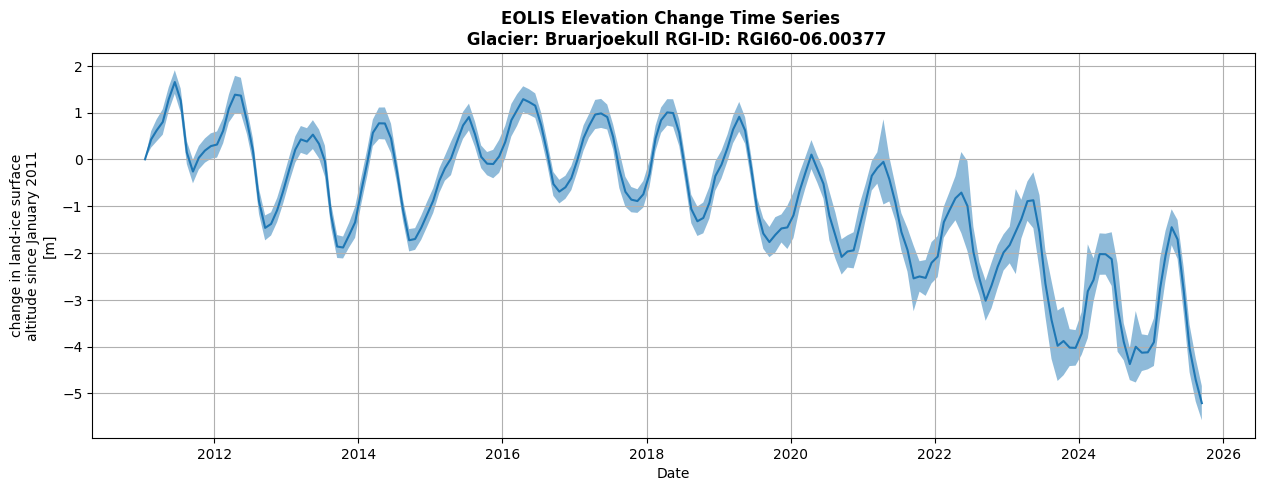
Glacier surface classification from Sentinel-2#
For DTC Glaciers, ENVEO provides a 10 m gridded glacier surface classification product derived from Sentinel-2 data. This dataset can be added to the L1 data cubes in the same way as shown above.
Variable |
Dims |
Description |
|---|---|---|
|
|
Glacier surface classification. |
|
|
Glacier surface classification uncertainty. |
|
|
Snowline altitude derived from glacier surface classification for three different snow cover area fractions (25%, 50% and 75%) per 30m elevation band. |
from dtcg.datacube.surface_type import DatacubeSurfaceType

dtcg_oggm_aut.add_data(DatacubeSurfaceType)

dtcg_oggm_aut.datacube_l1
<xarray.Dataset> Size: 79MB
Dimensions:                  (y: 229, x: 254, t_sfc_type: 82, snowcover_frac: 3)
Coordinates:
  * y                        (y) float32 916B 5.199e+06 5.199e+06 ... 5.187e+06
  * x                        (x) float32 1kB 6.321e+05 6.322e+05 ... 6.45e+05
  * t_sfc_type               (t_sfc_type) int64 656B 1435968000 ... 1632528000
  * snowcover_frac           (snowcover_frac) float64 24B 0.25 0.5 0.75
Data variables: (12/17)
    topo                     (y, x) float32 233kB 1.742e+03 ... 2.256e+03
    topo_smoothed            (y, x) float32 233kB 1.725e+03 ... 2.283e+03
    topo_valid_mask          (y, x) int8 58kB 1 1 1 1 1 1 1 1 ... 1 1 1 1 1 1 1
    glacier_mask             (y, x) int8 58kB 0 0 0 0 0 0 0 0 ... 0 0 0 0 0 0 0
    glacier_ext              (y, x) int8 58kB 0 0 0 0 0 0 0 0 ... 0 0 0 0 0 0 0
    consensus_ice_thickness  (y, x) float32 233kB nan nan nan ... nan nan nan
    ...                       ...
    millan_vx                (y, x) float32 233kB nan nan nan ... nan nan nan
    millan_vy                (y, x) float32 233kB nan nan nan ... nan nan nan
    hugonnet_dhdt            (y, x) float32 233kB 0.1893 0.1624 ... 0.001232
    sfc_type_data            (t_sfc_type, y, x) float64 38MB nan nan ... nan nan
    sfc_type_uncertainty     (t_sfc_type, y, x) float64 38MB nan nan ... nan nan
    sfc_type_snowline        (snowcover_frac, t_sfc_type) float64 2kB -inf .....
Attributes:
    author:              OGGM
    author_info:         Open Global Glacier Model
    pyproj_srs:          +proj=utm +zone=32 +datum=WGS84 +units=m +no_defs
    max_h_dem:           3737.275
    min_h_dem:           1701.9393
    max_h_glacier:       3574.82
    min_h_glacier:       2794.6978
    glacier_attributes:  {'rgi_id': 'RGI60-11.00719', 'glims_id': 'G010818E46...
RGI-ID: RGI60-11.00719- y: 229
- x: 254
- t_sfc_type: 82
- snowcover_frac: 3
- y(y)float325.199e+06 5.199e+06 ... 5.187e+06
- units :
- m
- long_name :
- y coordinate of projection
- standard_name :
- projection_y_coordinate
array([5.198700e+06, 5.198648e+06, 5.198598e+06, ..., 5.187174e+06, 5.187122e+06, 5.187072e+06], shape=(229,), dtype=float32) - x(x)float326.321e+05 6.322e+05 ... 6.45e+05
- units :
- m
- long_name :
- x coordinate of projection
- standard_name :
- projection_x_coordinate
array([632125.5, 632176.5, 632227.5, ..., 644926.5, 644977.5, 645028.5], shape=(254,), dtype=float32) - t_sfc_type(t_sfc_type)int641435968000 ... 1632528000
- long_name :
- Timestamp of surface type observations
- standard_name :
- time
- units :
- seconds since 1970-01-01 00:00:00
array([1435968000, 1438560000, 1439424000, 1440547200, 1445472000, 1463875200, 1467072000, 1468800000, 1470528000, 1472256000, 1473379200, 1474848000, 1476576000, 1477699200, 1494979200, 1495843200, 1497312000, 1498435200, 1499299200, 1500163200, 1501891200, 1502064000, 1503360000, 1503619200, 1504051200, 1505952000, 1529107200, 1529712000, 1530403200, 1531440000, 1531872000, 1532563200, 1532995200, 1534464000, 1534723200, 1535328000, 1537315200, 1537488000, 1537920000, 1556755200, 1558656000, 1559347200, 1559520000, 1560384000, 1560816000, 1561680000, 1563235200, 1563840000, 1566864000, 1567123200, 1567555200, 1568592000, 1569024000, 1569715200, 1590019200, 1591056000, 1591920000, 1593216000, 1594080000, 1594512000, 1595808000, 1596240000, 1596672000, 1596931200, 1597104000, 1597795200, 1597968000, 1599091200, 1599264000, 1599523200, 1599955200, 1600128000, 1628640000, 1628899200, 1629504000, 1630627200, 1630800000, 1631232000, 1631491200, 1631923200, 1632355200, 1632528000]) - snowcover_frac(snowcover_frac)float640.25 0.5 0.75
- long_name :
- Minimum snowcover fraction per elevation bin derived from surface type observations
array([0.25, 0.5 , 0.75])
- topo(y, x)float321.742e+03 1.719e+03 ... 2.256e+03
- units :
- m
- long_name :
- DEM topography
array([[1742.0565, 1718.5181, 1704.2761, ..., 2634.5364, 2637.226 , 2649.449 ], [1740.664 , 1714.4333, 1704.7688, ..., 2638.1663, 2647.0886, 2669.9976], [1736.8108, 1715.1503, 1707.2252, ..., 2642.6921, 2663.412 , 2690.577 ], ..., [2751.1343, 2759.4119, 2786.9155, ..., 2333.323 , 2293.8684, 2260.5007], [2716.279 , 2725.114 , 2737.6365, ..., 2320.2432, 2284.971 , 2255.3079], [2691.5476, 2701.3706, 2716.6023, ..., 2306.4504, 2277.612 , 2256.4653]], shape=(229, 254), dtype=float32) - topo_smoothed(y, x)float321.725e+03 1.719e+03 ... 2.283e+03
- units :
- m
- long_name :
- DEM topography smoothed with radius: 3e+02 m
array([[1724.8086, 1719.3458, 1712.1177, ..., 2636.773 , 2646.762 , 2652.9497], [1724.4166, 1719.1144, 1712.0779, ..., 2641.2793, 2652.6218, 2659.8135], [1724.0541, 1718.9253, 1712.0941, ..., 2649.7158, 2663.504 , 2672.4287], ..., [2769.0166, 2785.2014, 2816.7178, ..., 2337.9739, 2310.3232, 2294.3115], [2743.747 , 2758.433 , 2787.9717, ..., 2328.795 , 2302.123 , 2286.7192], [2729.0059, 2742.7756, 2771.012 , ..., 2323.2456, 2297.5151, 2282.7017]], shape=(229, 254), dtype=float32) - topo_valid_mask(y, x)int81 1 1 1 1 1 1 1 ... 1 1 1 1 1 1 1 1
- units :
- -
- long_name :
- DEM validity mask according to geotiff input (1-0)
array([[1, 1, 1, ..., 1, 1, 1], [1, 1, 1, ..., 1, 1, 1], [1, 1, 1, ..., 1, 1, 1], ..., [1, 1, 1, ..., 1, 1, 1], [1, 1, 1, ..., 1, 1, 1], [1, 1, 1, ..., 1, 1, 1]], shape=(229, 254), dtype=int8) - glacier_mask(y, x)int80 0 0 0 0 0 0 0 ... 0 0 0 0 0 0 0 0
- units :
- -
- long_name :
- Glacier mask
array([[0, 0, 0, ..., 0, 0, 0], [0, 0, 0, ..., 0, 0, 0], [0, 0, 0, ..., 0, 0, 0], ..., [0, 0, 0, ..., 0, 0, 0], [0, 0, 0, ..., 0, 0, 0], [0, 0, 0, ..., 0, 0, 0]], shape=(229, 254), dtype=int8) - glacier_ext(y, x)int80 0 0 0 0 0 0 0 ... 0 0 0 0 0 0 0 0
- units :
- -
- long_name :
- Glacier external boundaries
array([[0, 0, 0, ..., 0, 0, 0], [0, 0, 0, ..., 0, 0, 0], [0, 0, 0, ..., 0, 0, 0], ..., [0, 0, 0, ..., 0, 0, 0], [0, 0, 0, ..., 0, 0, 0], [0, 0, 0, ..., 0, 0, 0]], shape=(229, 254), dtype=int8) - consensus_ice_thickness(y, x)float32nan nan nan nan ... nan nan nan nan
- units :
- m
- long_name :
- Ice thickness from the consensus estimate
- base_url :
- https://cluster.klima.uni-bremen.de/~fmaussion/icevol/composite/
array([[nan, nan, nan, ..., nan, nan, nan], [nan, nan, nan, ..., nan, nan, nan], [nan, nan, nan, ..., nan, nan, nan], ..., [nan, nan, nan, ..., nan, nan, nan], [nan, nan, nan, ..., nan, nan, nan], [nan, nan, nan, ..., nan, nan, nan]], shape=(229, 254), dtype=float32) - itslive_v(y, x)float320.2434 0.2606 ... 0.2455 0.2186
- units :
- m yr-1
- long_name :
- ITS LIVE velocity data
array([[0.24344647, 0.26063082, 0.25035125, ..., 0.3579173 , 0.33561128, 0.28883582], [0.215022 , 0.23906074, 0.23105459, ..., 0.23957004, 0.2915858 , 0.25415778], [0.2174102 , 0.22514711, 0.21218726, ..., 0.19214211, 0.23711233, 0.22129242], ..., [0.12075873, 0.10186059, 0.1240496 , ..., 0.38581932, 0.2984355 , 0.27908072], [0.12112405, 0.08944868, 0.11879443, ..., 0.3723072 , 0.2577669 , 0.24903257], [0.2777302 , 0.29464224, 0.36886322, ..., 0.32898155, 0.2455291 , 0.21862198]], shape=(229, 254), dtype=float32) - itslive_vx(y, x)float320.1682 0.183 ... -0.02476 -0.05019
- units :
- m yr-1
- long_name :
- ITS LIVE velocity data in x map direction
array([[ 0.16823728, 0.18299547, 0.21395968, ..., 0.14311485, 0.18160792, 0.16164705], [ 0.21357566, 0.23756774, 0.23035474, ..., 0.23543918, 0.28862417, 0.25171182], [ 0.2174102 , 0.22514711, 0.21218726, ..., 0.19214211, 0.23711233, 0.22129242], ..., [ 0.09323441, 0.05910604, 0.06591155, ..., -0.09302186, -0.16451906, -0.21805006], [ 0.06243233, 0.00519245, 0.00568864, ..., -0.12723948, -0.18808964, -0.2339943 ], [ 0.07564991, 0.05815558, 0.06371289, ..., -0.04651477, -0.02475613, -0.05019299]], shape=(229, 254), dtype=float32) - itslive_vy(y, x)float32-0.09633 -0.09943 ... -0.05135 0.0
- units :
- m yr-1
- long_name :
- ITS LIVE velocity data in y map direction
array([[-0.09632614, -0.09943351, -0.04660948, ..., -0.22293597, -0.16981854, -0.14407717], [-0.00185245, -0.0019122 , -0.00089635, ..., -0.00428728, -0.00326578, -0.00277075], [ 0. , 0. , 0. , ..., 0. , 0. , 0. ], ..., [ 0. , 0. , 0. , ..., -0.31767195, -0.16941534, -0.08806729], [-0.01928749, -0.02240353, -0.02785993, ..., -0.26921242, -0.06118476, 0. ], [-0.2160203 , -0.25092 , -0.3120319 , ..., -0.2259387 , -0.0513498 , 0. ]], shape=(229, 254), dtype=float32) - millan_ice_thickness(y, x)float32nan nan nan nan ... nan nan nan nan
- units :
- m
- long_name :
- Ice thickness from Millan et al. 2022
- data_source :
- RGI-11_2021July09
array([[nan, nan, nan, ..., nan, nan, nan], [nan, nan, nan, ..., nan, nan, nan], [nan, nan, nan, ..., nan, nan, nan], ..., [nan, nan, nan, ..., nan, nan, nan], [nan, nan, nan, ..., nan, nan, nan], [nan, nan, nan, ..., nan, nan, nan]], shape=(229, 254), dtype=float32) - millan_v(y, x)float32nan nan nan nan ... nan nan nan nan
- units :
- m
- long_name :
- Ice velocity from Millan et al. 2022
- data_source :
- RGI-11_2021July01
array([[nan, nan, nan, ..., nan, nan, nan], [nan, nan, nan, ..., nan, nan, nan], [nan, nan, nan, ..., nan, nan, nan], ..., [nan, nan, nan, ..., nan, nan, nan], [nan, nan, nan, ..., nan, nan, nan], [nan, nan, nan, ..., nan, nan, nan]], shape=(229, 254), dtype=float32) - millan_vx(y, x)float32nan nan nan nan ... nan nan nan nan
- units :
- m
- long_name :
- Ice velocity in map x direction from Millan et al. 2022
- data_source :
- RGI-11_2021July01
array([[nan, nan, nan, ..., nan, nan, nan], [nan, nan, nan, ..., nan, nan, nan], [nan, nan, nan, ..., nan, nan, nan], ..., [nan, nan, nan, ..., nan, nan, nan], [nan, nan, nan, ..., nan, nan, nan], [nan, nan, nan, ..., nan, nan, nan]], shape=(229, 254), dtype=float32) - millan_vy(y, x)float32nan nan nan nan ... nan nan nan nan
- units :
- m
- long_name :
- Ice velocity in map y direction from Millan et al. 2022
- data_source :
- RGI-11_2021July01
array([[nan, nan, nan, ..., nan, nan, nan], [nan, nan, nan, ..., nan, nan, nan], [nan, nan, nan, ..., nan, nan, nan], ..., [nan, nan, nan, ..., nan, nan, nan], [nan, nan, nan, ..., nan, nan, nan], [nan, nan, nan, ..., nan, nan, nan]], shape=(229, 254), dtype=float32) - hugonnet_dhdt(y, x)float320.1893 0.1624 ... 0.004438 0.001232
- units :
- m
- long_name :
- dhdt (2000-2020) from Hugonnet et al. 2021
- data_source :
- /home/data/download/cluster.klima.uni-bremen.de/~oggm/geodetic_ref_mb_maps/dhdt/N46E010_2000-01-01_2020-01-01_dhdt.tif
array([[ 1.8931952e-01, 1.6242915e-01, 1.4414129e-01, ..., -1.1726944e+00, -8.4028047e-01, -5.2263099e-01], [ 1.9792432e-01, 1.8828717e-01, 3.7784296e-01, ..., -1.0144438e+00, -6.3453114e-01, -3.5095587e-01], [ 2.0982631e-01, 2.2902362e-01, 6.1095959e-01, ..., -8.5337508e-01, -4.3152189e-01, -1.8335494e-01], ..., [-8.4933359e-03, -2.2932557e-02, -2.3965480e-02, ..., -7.7997725e-03, -7.1713943e-03, -5.7778261e-03], [-3.8133018e-02, -3.8725853e-02, -2.9151555e-02, ..., -9.8316406e-04, 4.3411115e-03, 3.5339131e-03], [-6.1521191e-02, -7.7394404e-02, -6.3811660e-02, ..., -1.6706563e-04, 4.4379705e-03, 1.2322172e-03]], shape=(229, 254), dtype=float32) - sfc_type_data(t_sfc_type, y, x)float64nan nan nan nan ... nan nan nan nan
- long_name :
- Glacier surface classification
- data_source :
- ENVEO
- units :
- none
- code_description :
- Extract dict with eval(ds.code).
- code :
- {0: 'unclassified', 1: 'snow', 2: 'firn / old snow / bright ice', 3: 'clean ice', 4: 'debris', 5: 'cloud', 'nan': 'no data'}
array([[[nan, nan, nan, ..., nan, nan, nan], [nan, nan, nan, ..., nan, nan, nan], [nan, nan, nan, ..., nan, nan, nan], ..., [nan, nan, nan, ..., nan, nan, nan], [nan, nan, nan, ..., nan, nan, nan], [nan, nan, nan, ..., nan, nan, nan]], [[nan, nan, nan, ..., nan, nan, nan], [nan, nan, nan, ..., nan, nan, nan], [nan, nan, nan, ..., nan, nan, nan], ..., [nan, nan, nan, ..., nan, nan, nan], [nan, nan, nan, ..., nan, nan, nan], [nan, nan, nan, ..., nan, nan, nan]], [[nan, nan, nan, ..., nan, nan, nan], [nan, nan, nan, ..., nan, nan, nan], [nan, nan, nan, ..., nan, nan, nan], ..., ... ..., [nan, nan, nan, ..., nan, nan, nan], [nan, nan, nan, ..., nan, nan, nan], [nan, nan, nan, ..., nan, nan, nan]], [[nan, nan, nan, ..., nan, nan, nan], [nan, nan, nan, ..., nan, nan, nan], [nan, nan, nan, ..., nan, nan, nan], ..., [nan, nan, nan, ..., nan, nan, nan], [nan, nan, nan, ..., nan, nan, nan], [nan, nan, nan, ..., nan, nan, nan]], [[nan, nan, nan, ..., nan, nan, nan], [nan, nan, nan, ..., nan, nan, nan], [nan, nan, nan, ..., nan, nan, nan], ..., [nan, nan, nan, ..., nan, nan, nan], [nan, nan, nan, ..., nan, nan, nan], [nan, nan, nan, ..., nan, nan, nan]]], shape=(82, 229, 254)) - sfc_type_uncertainty(t_sfc_type, y, x)float64nan nan nan nan ... nan nan nan nan
- long_name :
- Glacier surface classification uncertainty
- data_source :
- ENVEO
- units :
- none
- code_description :
- Extract dict with eval(ds.code).
- code :
- {1: 'low uncertainty for illuminated pixel', 2: 'medium uncertainty for illuminated pixel', 3: 'high uncertainty for illuminated pixel', 5: 'cloud', 11: 'low uncertainty for shaded pixel', 12: 'medium uncertainty for shaded pixel', 13: 'high uncertainty for shaded pixel', 'nan': 'no data'}
array([[[nan, nan, nan, ..., nan, nan, nan], [nan, nan, nan, ..., nan, nan, nan], [nan, nan, nan, ..., nan, nan, nan], ..., [nan, nan, nan, ..., nan, nan, nan], [nan, nan, nan, ..., nan, nan, nan], [nan, nan, nan, ..., nan, nan, nan]], [[nan, nan, nan, ..., nan, nan, nan], [nan, nan, nan, ..., nan, nan, nan], [nan, nan, nan, ..., nan, nan, nan], ..., [nan, nan, nan, ..., nan, nan, nan], [nan, nan, nan, ..., nan, nan, nan], [nan, nan, nan, ..., nan, nan, nan]], [[nan, nan, nan, ..., nan, nan, nan], [nan, nan, nan, ..., nan, nan, nan], [nan, nan, nan, ..., nan, nan, nan], ..., ... ..., [nan, nan, nan, ..., nan, nan, nan], [nan, nan, nan, ..., nan, nan, nan], [nan, nan, nan, ..., nan, nan, nan]], [[nan, nan, nan, ..., nan, nan, nan], [nan, nan, nan, ..., nan, nan, nan], [nan, nan, nan, ..., nan, nan, nan], ..., [nan, nan, nan, ..., nan, nan, nan], [nan, nan, nan, ..., nan, nan, nan], [nan, nan, nan, ..., nan, nan, nan]], [[nan, nan, nan, ..., nan, nan, nan], [nan, nan, nan, ..., nan, nan, nan], [nan, nan, nan, ..., nan, nan, nan], ..., [nan, nan, nan, ..., nan, nan, nan], [nan, nan, nan, ..., nan, nan, nan], [nan, nan, nan, ..., nan, nan, nan]]], shape=(82, 229, 254)) - sfc_type_snowline(snowcover_frac, t_sfc_type)float64-inf 3.09e+03 ... nan 3.09e+03
- long_name :
- Snowline altitude derived from glacier surface classification
- data_source :
- ENVEO
- units :
- m
- inf_values :
- {inf: 3570.0, -inf: 2760.0}
array([[ -inf, 3090., 3120., 3180.,  -inf,  -inf,  -inf,  -inf,  -inf,
        3120., 2880.,  -inf,  -inf,  -inf,  -inf,  -inf,  -inf,  -inf,
        3000., 2970., 3270., 3120., 3090., 3390.,   inf,  -inf,  -inf,
         -inf,   nan, 3000., 3030.,   nan, 3120., 3240., 3120.,  -inf,
        3390., 3420., 3420.,  -inf,  -inf,  -inf,  -inf,  -inf,  -inf,
         -inf, 2880.,  -inf, 3180., 3360., 3240., 2940., 3180., 2910.,
         -inf,  -inf,  -inf,  -inf,  -inf, 2880., 3000., 3030., 2910.,
        3060., 3090., 3090., 3120., 2910., 3090., 3090., 3240., 3240.,
          nan, 3120., 3120.,   nan, 2940., 3000., 3120., 3180.,   nan,
        2940.],
       [ -inf, 3120., 3210., 3240.,  -inf,  -inf,  -inf,  -inf,  -inf,
        3240., 2910.,  -inf,  -inf,  -inf,  -inf,  -inf,  -inf, 3000.,
        3030., 3000.,   inf, 3180., 3120.,   inf,   inf,  -inf,  -inf,
         -inf,   nan, 3030., 3060.,   nan, 3210.,   inf,   inf, 2940.,
        3390., 3420.,   inf,  -inf,  -inf,  -inf,  -inf,  -inf,  -inf,
         -inf, 2880., 2880., 3240.,   inf, 3420., 3000., 3270., 2940.,
         -inf,  -inf,  -inf,  -inf, 2880., 2940., 3030., 3090., 2940.,
        3090., 3120., 3120., 3240., 2940., 3120., 3120., 3420., 3420.,
          nan, 3180., 3180.,   nan, 3000., 3090., 3180., 3240.,   nan,
        2970.],
       [ -inf, 3210., 3420., 3390.,  -inf,  -inf,  -inf,  -inf,  -inf,
        3420.,   inf,  -inf,  -inf,  -inf,  -inf,  -inf,  -inf, 3030.,
        3060., 3060.,   inf, 3180., 3180.,   inf,   inf,  -inf,  -inf,
         -inf,   nan, 3060., 3090.,   nan, 3300.,   inf,   inf, 2970.,
        3420.,   inf,   inf,  -inf,  -inf,  -inf,  -inf,  -inf,  -inf,
         -inf, 2940., 2970., 3420.,   inf, 3420., 3090., 3420., 2940.,
         -inf,  -inf,  -inf,  -inf, 2940., 2940., 3060., 3120., 2940.,
        3240., 3390., 3420., 3420., 2940., 3240., 3150., 3420., 3450.,
          nan, 3240., 3270.,   nan, 3060., 3120., 3270., 3390.,   nan,
        3090.]])
- author :
- OGGM
- author_info :
- Open Global Glacier Model
- pyproj_srs :
- +proj=utm +zone=32 +datum=WGS84 +units=m +no_defs
- max_h_dem :
- 3737.275
- min_h_dem :
- 1701.9393
- max_h_glacier :
- 3574.82
- min_h_glacier :
- 2794.6978
- glacier_attributes :
- {'rgi_id': 'RGI60-11.00719', 'glims_id': 'G010818E46876N', 'cenlon': 10.818, 'cenlat': 46.8762, 'rgi_region': '11', 'rgi_subregion': '11-01', 'rgi_version': '60', 'rgi_dem_source': 'COPDEM30', 'glacier_type': 'Glacier', 'terminus_type': 'Land-terminating', 'name': 'Vernagtferner', 'rgi_region_name': '11: Central Europe', 'rgi_subregion_name': '11-01: Alps ', 'rgi_date': 2003}
- RGI-ID :
- RGI60-11.00719
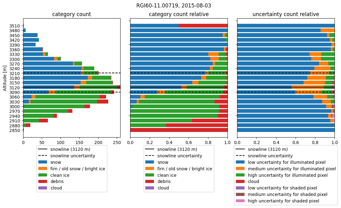
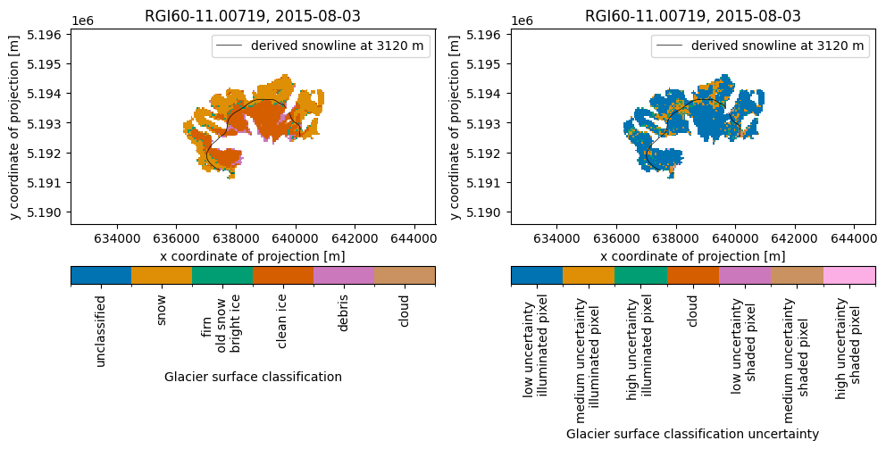
The snowline was derived within DTC Glaciers for model validation and could also be assimilated in the future. To derive it, we aggregated the gridded glacier surface classification into 30 m elevation bands and calculated the snow cover area fraction for each band, excluding cloud-covered pixels.
We then identified the lowest elevation band where one of the three thresholds - 25%, 50%, or 75% - was exceeded for the first time.
Let’s look at one example:
Show code cell source
Hide code cell source
import numpy as np
import xarray as xr
from dtcg.datacube.surface_type import (
    get_categories_per_elevation_band,
    exclude_empty_elevation_bins,
    exclude_dates_with_too_much_cloud_cover,
    get_snowline,
)


def plot_surface_classification_per_elev_band(datacube_l1, date):
    ds_obs = get_categories_per_elevation_band(datacube_l1)
    ds_obs = exclude_empty_elevation_bins(ds=ds_obs)
    ds_obs = exclude_dates_with_too_much_cloud_cover(ds=ds_obs)

    ds_use = ds_obs.sel(t_sfc_type=date)
    ds_use = xr.decode_cf(ds_use)

    bin_idx, bin_elev = get_snowline(ds_use)

    fig, axs = plt.subplots(1, 3, figsize=(13, 5), gridspec_kw={"wspace": 0.1})

    ax_total = axs[0]
    ax_relative = axs[1]
    ax_uncertainty = axs[2]

    def plot_horizontal_stacked_bar(ax, ds, categories, var, normalize=False):
        category_dict = eval(
            ds[categories].attrs["code"]
        )  # ast.literal_eval(ds[categories].attrs['code'])
        previous_values = None
        for category in ds_use[categories]:
            current_values = ds.loc[{categories: category}][var].values
            if normalize:
                number_grid_points_elev_bin = ds.category_counts.sum(dim="category")
                current_values = (
                    current_values.astype(float) / number_grid_points_elev_bin
                )
            ax.barh(
                ds.elevation_bin,
                current_values,
                left=previous_values,
                label=category_dict[int(category)],
            )

            if previous_values is None:
                previous_values = current_values
            else:
                previous_values = previous_values + current_values

        ax.invert_yaxis()

    plot_horizontal_stacked_bar(ax_total, ds_use, "category", "category_counts")
    plot_horizontal_stacked_bar(
        ax_relative, ds_use, "category", "category_counts", normalize=True
    )
    plot_horizontal_stacked_bar(
        ax_uncertainty, ds_use, "uncertainty_flag", "uncertainty_counts", normalize=True
    )

    def add_snowline(ax):
        if np.isneginf(bin_elev[1]):
            extra_label = "fully snow covered"
        elif np.isposinf(bin_elev[1]):
            extra_label = "fully snow free"
        else:
            extra_label = f"{bin_elev[1]:.0f} m"
        ax.axhline(bin_idx[0], color="k", linestyle="--")
        ax.axhline(
            bin_idx[1], color="k", linestyle="-", label=f"snowline ({extra_label})"
        )
        ax.axhline(bin_idx[2], color="k", linestyle="--", label="snowline uncertainty")

    def set_legend(ax):
        ax.legend(loc="upper center", bbox_to_anchor=(0.5, -0.05))

    ax_total.set_yticks(
        ds_use.elevation_bin, [int(elev) for elev in ds_use.lower_elevation.values]
    )
    ax_total.set_ylabel("Altitude [m]")
    ax_total.set_title("category count")
    add_snowline(ax_total)
    set_legend(ax_total)

    ax_relative.set_title("category count relative")
    ax_relative.set_yticklabels([])
    add_snowline(ax_relative)
    set_legend(ax_relative)

    ax_uncertainty.set_title("uncertainty count relative")
    ax_uncertainty.set_yticklabels([])
    add_snowline(ax_uncertainty)
    set_legend(ax_uncertainty)

    fig.suptitle(
        f"{datacube_l1.attrs['RGI-ID']}, {np.datetime_as_string(ds_use.t_sfc_type.values, unit='D')}"
    )

    plt.show()
plot_surface_classification_per_elev_band(
    datacube_l1=dtcg_oggm_aut.datacube_l1, date=dtcg_oggm_aut.datacube_l1.t_sfc_type[1]
)
Let’s visualize the derived snowline on top of the original gridded data:
Show code cell source
Hide code cell source
import matplotlib.pyplot as plt
import matplotlib.colors as mcolors
import seaborn as sns
import matplotlib.lines as mlines


def build_categorical_colormap(class_labels, palette_name="colorblind"):

    # Extract integer classes and sort them
    classes = sorted(
        [k for k in class_labels.keys() if isinstance(k, (int, np.integer))]
    )
    n = len(classes)

    # Pick n colors from seaborn palette
    colors = sns.color_palette(palette_name, n)

    # Create colormap
    cmap = mcolors.ListedColormap(colors)

    # Set NaN color ("bad" values)
    # cmap.set_bad("lightgray")

    # Boundaries between classes — last boundary is +1
    bounds = [c - 0.5 for c in classes] + [classes[-1] + 0.5]
    norm = mcolors.BoundaryNorm(bounds, cmap.N)

    return norm, cmap, classes


def plot_gridded_surface_classification(
    datacube_l1, date, x_zoom=70, y_zoom=50, snowline=None
):

    ds_plot = datacube_l1.isel(
        x=slice(x_zoom, len(datacube_l1.x) - x_zoom),
        y=slice(y_zoom, len(datacube_l1.y) - y_zoom),
    )

    ds_plot = ds_plot.sel(t_sfc_type=date)
    ds_plot = xr.decode_cf(ds_plot)

    # Integer classes in your dataset
    dict_labels_1 = {
        0: "unclassified",
        1: "snow",
        2: "firn \n old snow \n bright ice",
        3: "clean ice",
        4: "debris",
        5: "cloud",
        "nan": "no data",
    }  # ast.literal_eval(ds_plot.sfc_type_data.code)

    dict_labels_2 = {
        1: "low uncertainty \n illuminated pixel",
        2: "medium uncertainty \n illuminated pixel",
        3: "high uncertainty \n illuminated pixel",
        5: "cloud",
        11: "low uncertainty \n shaded pixel",
        12: "medium uncertainty \n shaded pixel",
        13: "high uncertainty \n shaded pixel",
        "nan": "no data",
    }  # ast.literal_eval(ds_plot.sfc_type_uncertainty.code)

    norm_1, cmap_1, classes_1 = build_categorical_colormap(dict_labels_1)
    norm_2, cmap_2, classes_2 = build_categorical_colormap(dict_labels_2)

    # Your data array
    da_1 = ds_plot.where(ds_plot.glacier_mask).sfc_type_data
    da_2 = ds_plot.where(ds_plot.glacier_mask).sfc_type_uncertainty

    fig, axs = plt.subplots(1, 2, figsize=(10, 5))

    ax_1 = axs[0]
    ax_2 = axs[1]

    mappable_1 = da_1.plot(ax=ax_1, cmap=cmap_1, norm=norm_1, add_colorbar=False)
    mappable_2 = da_2.plot(ax=ax_2, cmap=cmap_2, norm=norm_2, add_colorbar=False)

    # add derived snowline

    cs = ds_plot.where(ds_plot.glacier_mask).topo_smoothed.plot.contour(
        ax=ax_1, levels=[snowline], colors="k", linewidths=0.5
    )
    proxy = mlines.Line2D(
        [], [], color="k", linewidth=0.5, label=f"derived snowline at {snowline} m"
    )
    ax_1.legend(handles=[proxy])

    cs = ds_plot.where(ds_plot.glacier_mask).topo_smoothed.plot.contour(
        ax=ax_2, levels=[snowline], colors="k", linewidths=0.5
    )
    proxy_2 = mlines.Line2D(
        [], [], color="k", linewidth=0.5, label=f"derived snowline at {snowline} m"
    )
    ax_2.legend(handles=[proxy_2])

    # Add labeled colorbar
    cbar_1 = plt.colorbar(
        mappable_1, ax=ax_1, orientation="horizontal", ticks=classes_1
    )
    cbar_1.ax.set_xticklabels([f"{dict_labels_1[c]}" for c in classes_1], rotation=90)
    cbar_1.set_label(ds_plot.sfc_type_data.long_name)

    cbar_2 = plt.colorbar(
        mappable_2,
        ax=ax_2,
        ticks=[1, 2, 3.5, 7.5, 11, 12, 13],
        orientation="horizontal",
    )  # classes_2)
    cbar_2.ax.set_xticklabels([f"{dict_labels_2[c]}" for c in classes_2], rotation=90)
    cbar_2.set_label(ds_plot.sfc_type_uncertainty.long_name)

    ax_1.axis("equal")
    ax_2.axis("equal")

    ax_1.set_title(
        f"{datacube_l1.attrs['RGI-ID']}, {np.datetime_as_string(da_1.t_sfc_type.values, unit='D')}"
    )
    ax_2.set_title(
        f"{datacube_l1.attrs['RGI-ID']}, {np.datetime_as_string(da_2.t_sfc_type.values, unit='D')}"
    )

    fig.tight_layout()
    plt.show()
plot_gridded_surface_classification(
    datacube_l1=dtcg_oggm_aut.datacube_l1,
    date=dtcg_oggm_aut.datacube_l1.t_sfc_type[1],
    snowline=3120,
)
In-situ mass balance observations from WGMS#
For validation, the DTCG API can add in-situ mass balance observations from WGMS to the L1 data cubes for glaciers where such observations are available, using the same approach as shown above.
Variable |
Dims |
Description |
|---|---|---|
|
|
Specific mass balance observation as reported tothe World Glacier Monitoring Service. |
|
|
Specific mass balance observation uncertainty as reported to the World Glacier Monitoring Service. If no value was reported it is set to 200 mm w.e.. |
from dtcg.datacube.wgms import DatacubeWGMS

dtcg_oggm_ice.add_data(DatacubeWGMS)

dtcg_oggm_ice.datacube_l1
<xarray.Dataset> Size: 464MB
Dimensions:                                  (y: 370, x: 436, t: 177, t_wgms: 32)
Coordinates:
  * y                                        (y) float32 1kB 7.201e+06 ... 7....
  * x                                        (x) float32 2kB 3.94e+05 ... 4.8...
  * t                                        (t) int64 1kB 1295049600 ... 175...
  * t_wgms                                   (t_wgms) int64 256B 1993 ... 2024
    spatial_ref                              int64 8B 0
Data variables: (12/20)
    topo                                     (y, x) float32 645kB 1.147e+03 ....
    topo_smoothed                            (y, x) float32 645kB 1.151e+03 ....
    topo_valid_mask                          (y, x) int8 161kB 1 1 1 1 ... 1 1 1
    glacier_mask                             (y, x) int8 161kB 0 0 0 0 ... 0 0 0
    glacier_ext                              (y, x) int8 161kB 0 0 0 0 ... 0 0 0
    consensus_ice_thickness                  (y, x) float32 645kB nan ... nan
    ...                                       ...
    eolis_gridded_elevation_change           (t, y, x) float64 228MB nan ... nan
    eolis_gridded_elevation_change_sigma     (t, y, x) float64 228MB nan ... nan
    eolis_elevation_change_timeseries        (t) float64 1kB 0.0 ... -5.208
    eolis_elevation_change_sigma_timeseries  (t) float64 1kB 0.0 ... 0.3651
    wgms_mb                                  (t_wgms) float64 256B 1.09e+03 ....
    wgms_mb_unc                              (t_wgms) float64 256B 200.0 ... ...
Attributes:
    author:              OGGM
    author_info:         Open Global Glacier Model
    pyproj_srs:          +proj=utm +zone=28 +datum=WGS84 +units=m +no_defs
    max_h_dem:           1901.579
    min_h_dem:           -0.24698931
    max_h_glacier:       1875.962
    min_h_glacier:       623.5142
    glacier_attributes:  {'rgi_id': 'RGI60-06.00377', 'glims_id': 'G343733E64...
RGI-ID: RGI60-06.00377- y: 370
- x: 436
- t: 177
- t_wgms: 32
- y(y)float327.201e+06 7.201e+06 ... 7.127e+06
- units :
- m
- long_name :
- y coordinate of projection
- standard_name :
- projection_y_coordinate
array([7.200982e+06, 7.200782e+06, 7.200582e+06, ..., 7.127582e+06, 7.127382e+06, 7.127182e+06], shape=(370,), dtype=float32) - x(x)float323.94e+05 3.942e+05 ... 4.81e+05
- units :
- m
- long_name :
- x coordinate of projection
- standard_name :
- projection_x_coordinate
array([393962.1, 394162.1, 394362.1, ..., 480562.1, 480762.1, 480962.1], shape=(436,), dtype=float32) - t(t)int641295049600 ... 1757894400
- standard_name :
- time
- long_name :
- time since the unix epoch
- units :
- seconds since 1970-01-01 00:00:00
array([1295049600, 1297728000, 1300147200, 1302825600, 1305417600, 1308096000, 1310688000, 1313366400, 1316044800, 1318636800, 1321315200, 1323907200, 1326585600, 1329264000, 1331769600, 1334448000, 1337040000, 1339718400, 1342310400, 1344988800, 1347667200, 1350259200, 1352937600, 1355529600, 1358208000, 1360886400, 1363305600, 1365984000, 1368576000, 1371254400, 1373846400, 1376524800, 1379203200, 1381795200, 1384473600, 1387065600, 1389744000, 1392422400, 1394841600, 1397520000, 1400112000, 1402790400, 1405382400, 1408060800, 1410739200, 1413331200, 1416009600, 1418601600, 1421280000, 1423958400, 1426377600, 1429056000, 1431648000, 1434326400, 1436918400, 1439596800, 1442275200, 1444867200, 1447545600, 1450137600, 1452816000, 1455494400, 1458000000, 1460678400, 1463270400, 1465948800, 1468540800, 1471219200, 1473897600, 1476489600, 1479168000, 1481760000, 1484438400, 1487116800, 1489536000, 1492214400, 1494806400, 1497484800, 1500076800, 1502755200, 1505433600, 1508025600, 1510704000, 1513296000, 1515974400, 1518652800, 1521072000, 1523750400, 1526342400, 1529020800, 1531612800, 1534291200, 1536969600, 1539561600, 1542240000, 1544832000, 1547510400, 1550188800, 1552608000, 1555286400, 1557878400, 1560556800, 1563148800, 1565827200, 1568505600, 1571097600, 1573776000, 1576368000, 1579046400, 1581724800, 1584230400, 1586908800, 1589500800, 1592179200, 1594771200, 1597449600, 1600128000, 1602720000, 1605398400, 1607990400, 1610668800, 1613347200, 1615766400, 1618444800, 1621036800, 1623715200, 1626307200, 1628985600, 1631664000, 1634256000, 1636934400, 1639526400, 1642204800, 1644883200, 1647302400, 1649980800, 1652572800, 1655251200, 1657843200, 1660521600, 1663200000, 1665792000, 1668470400, 1671062400, 1673740800, 1676419200, 1678838400, 1681516800, 1684108800, 1686787200, 1689379200, 1692057600, 1694736000, 1697328000, 1700006400, 1702598400, 1705276800, 1707955200, 1710460800, 1713139200, 1715731200, 1718409600, 1721001600, 1723680000, 1726358400, 1728950400, 1731628800, 1734220800, 1736899200, 1739577600, 1741996800, 1744675200, 1747267200, 1749945600, 1752537600, 1755216000, 1757894400]) - t_wgms(t_wgms)int641993 1994 1995 ... 2022 2023 2024
array([1993, 1994, 1995, 1996, 1997, 1998, 1999, 2000, 2001, 2002, 2003, 2004, 2005, 2006, 2007, 2008, 2009, 2010, 2011, 2012, 2013, 2014, 2015, 2016, 2017, 2018, 2019, 2020, 2021, 2022, 2023, 2024]) - spatial_ref()int640
- crs_wkt :
- PROJCS["unknown",GEOGCS["unknown",DATUM["WGS_1984",SPHEROID["WGS 84",6378137,298.257223563,AUTHORITY["EPSG","7030"]],AUTHORITY["EPSG","6326"]],PRIMEM["Greenwich",0,AUTHORITY["EPSG","8901"]],UNIT["degree",0.0174532925199433,AUTHORITY["EPSG","9122"]]],PROJECTION["Transverse_Mercator"],PARAMETER["latitude_of_origin",0],PARAMETER["central_meridian",-15],PARAMETER["scale_factor",0.9996],PARAMETER["false_easting",500000],PARAMETER["false_northing",0],UNIT["metre",1,AUTHORITY["EPSG","9001"]],AXIS["Easting",EAST],AXIS["Northing",NORTH]]
- semi_major_axis :
- 6378137.0
- semi_minor_axis :
- 6356752.314245179
- inverse_flattening :
- 298.257223563
- reference_ellipsoid_name :
- WGS 84
- longitude_of_prime_meridian :
- 0.0
- prime_meridian_name :
- Greenwich
- geographic_crs_name :
- unknown
- horizontal_datum_name :
- World Geodetic System 1984
- projected_crs_name :
- unknown
- grid_mapping_name :
- transverse_mercator
- latitude_of_projection_origin :
- 0.0
- longitude_of_central_meridian :
- -15.0
- false_easting :
- 500000.0
- false_northing :
- 0.0
- scale_factor_at_central_meridian :
- 0.9996
- spatial_ref :
- PROJCS["unknown",GEOGCS["unknown",DATUM["WGS_1984",SPHEROID["WGS 84",6378137,298.257223563,AUTHORITY["EPSG","7030"]],AUTHORITY["EPSG","6326"]],PRIMEM["Greenwich",0,AUTHORITY["EPSG","8901"]],UNIT["degree",0.0174532925199433,AUTHORITY["EPSG","9122"]]],PROJECTION["Transverse_Mercator"],PARAMETER["latitude_of_origin",0],PARAMETER["central_meridian",-15],PARAMETER["scale_factor",0.9996],PARAMETER["false_easting",500000],PARAMETER["false_northing",0],UNIT["metre",1,AUTHORITY["EPSG","9001"]],AXIS["Easting",EAST],AXIS["Northing",NORTH]]
array(0)
- topo(y, x)float321.147e+03 1.141e+03 ... 0.0 0.0
- units :
- m
- long_name :
- DEM topography
array([[1.1469581e+03, 1.1407299e+03, 1.1381298e+03, ..., 6.6475842e+02, 6.5947559e+02, 6.5525848e+02], [1.1705750e+03, 1.1692976e+03, 1.1588870e+03, ..., 6.6196667e+02, 6.5631232e+02, 6.5455737e+02], [1.2064128e+03, 1.2036810e+03, 1.1891963e+03, ..., 6.5896118e+02, 6.5506055e+02, 6.5444885e+02], ..., [8.8076691e+02, 8.6122577e+02, 8.8352625e+02, ..., 2.6724836e-01, 1.7347394e-01, 1.9891816e-01], [8.6362506e+02, 8.5418347e+02, 8.8737177e+02, ..., 0.0000000e+00, 0.0000000e+00, 0.0000000e+00], [8.4890240e+02, 8.5093469e+02, 8.8949481e+02, ..., 0.0000000e+00, 0.0000000e+00, 0.0000000e+00]], shape=(370, 436), dtype=float32) - topo_smoothed(y, x)float321.151e+03 1.147e+03 ... 0.0002844
- units :
- m
- long_name :
- DEM topography smoothed with radius: 3e+02 m
array([[1.1508660e+03, 1.1469803e+03, 1.1412454e+03, ..., 6.6404663e+02, 6.5915826e+02, 6.5589307e+02], [1.1726067e+03, 1.1690500e+03, 1.1603943e+03, ..., 6.6184216e+02, 6.5738916e+02, 6.5511414e+02], [1.2069194e+03, 1.2019698e+03, 1.1898363e+03, ..., 6.5961139e+02, 6.5609778e+02, 6.5490656e+02], ..., [8.7737811e+02, 8.7143109e+02, 8.8398639e+02, ..., 1.9621927e-01, 1.4236444e-01, 1.5236741e-01], [8.6219836e+02, 8.6371283e+02, 8.8232770e+02, ..., 1.7820445e-01, 4.1718520e-02, 4.0628150e-02], [8.5193823e+02, 8.5963940e+02, 8.8198364e+02, ..., 1.4999704e-01, 9.4814815e-05, 2.8444445e-04]], shape=(370, 436), dtype=float32) - topo_valid_mask(y, x)int81 1 1 1 1 1 1 1 ... 1 1 1 1 1 1 1 1
- units :
- -
- long_name :
- DEM validity mask according to geotiff input (1-0)
array([[1, 1, 1, ..., 1, 1, 1], [1, 1, 1, ..., 1, 1, 1], [1, 1, 1, ..., 1, 1, 1], ..., [1, 1, 1, ..., 1, 1, 1], [1, 1, 1, ..., 1, 1, 1], [1, 1, 1, ..., 1, 1, 1]], shape=(370, 436), dtype=int8) - glacier_mask(y, x)int80 0 0 0 0 0 0 0 ... 0 0 0 0 0 0 0 0
- units :
- -
- long_name :
- Glacier mask
array([[0, 0, 0, ..., 0, 0, 0], [0, 0, 0, ..., 0, 0, 0], [0, 0, 0, ..., 0, 0, 0], ..., [0, 0, 0, ..., 0, 0, 0], [0, 0, 0, ..., 0, 0, 0], [0, 0, 0, ..., 0, 0, 0]], shape=(370, 436), dtype=int8) - glacier_ext(y, x)int80 0 0 0 0 0 0 0 ... 0 0 0 0 0 0 0 0
- units :
- -
- long_name :
- Glacier external boundaries
array([[0, 0, 0, ..., 0, 0, 0], [0, 0, 0, ..., 0, 0, 0], [0, 0, 0, ..., 0, 0, 0], ..., [0, 0, 0, ..., 0, 0, 0], [0, 0, 0, ..., 0, 0, 0], [0, 0, 0, ..., 0, 0, 0]], shape=(370, 436), dtype=int8) - consensus_ice_thickness(y, x)float32nan nan nan nan ... nan nan nan nan
- units :
- m
- long_name :
- Ice thickness from the consensus estimate
- base_url :
- https://cluster.klima.uni-bremen.de/~fmaussion/icevol/composite/
array([[nan, nan, nan, ..., nan, nan, nan], [nan, nan, nan, ..., nan, nan, nan], [nan, nan, nan, ..., nan, nan, nan], ..., [nan, nan, nan, ..., nan, nan, nan], [nan, nan, nan, ..., nan, nan, nan], [nan, nan, nan, ..., nan, nan, nan]], shape=(370, 436), dtype=float32) - itslive_v(y, x)float320.2549 0.316 0.104 ... nan nan nan
- units :
- m yr-1
- long_name :
- ITS LIVE velocity data
array([[0.2548638 , 0.3160016 , 0.1039561 , ..., 0.9141536 , 0.8403372 , 0.69694364], [0.27767682, 0.24819988, 0.28476351, ..., 2.0485506 , 1.150246 , 0.50836325], [0.24675122, 0.27259168, 0.39868486, ..., 1.292929 , 0.61550474, 0.7452541 ], ..., [2.608234 , 1.8436593 , 2.698295 , ..., 0.37593848, 0.3458429 , 0.17436156], [1.7304813 , 1.645862 , 2.7974434 , ..., 0.331727 , 0.3038549 , nan], [2.200289 , 1.1182725 , 1.0266634 , ..., nan, nan, nan]], shape=(370, 436), dtype=float32) - itslive_vx(y, x)float320.09866 -0.03163 ... nan nan
- units :
- m yr-1
- long_name :
- ITS LIVE velocity data in x map direction
array([[ 0.09866323, -0.03163351, 0.01193277, ..., 0.43653226, 0.27403608, 0.6505354 ], [ 0.13080858, -0.05709021, -0.10543129, ..., 1.1964303 , 0.8653776 , 0.37876108], [-0.00792862, -0.09918541, 0.02574821, ..., 1.2704426 , 0.5189546 , 0.54376847], ..., [ 2.0647523 , 1.4015841 , 1.7450721 , ..., 0.1196125 , 0.07965311, 0.15799367], [ 0.7335261 , 0.9962476 , 1.6772281 , ..., 0.22557321, -0.0558848 , nan], [-0.40105644, 0.01473092, 0.09578909, ..., nan, nan, nan]], shape=(370, 436), dtype=float32) - itslive_vy(y, x)float320.2295 0.2614 -0.03591 ... nan nan
- units :
- m yr-1
- long_name :
- ITS LIVE velocity data in y map direction
array([[ 0.22947061, 0.26136097, -0.03591328, ..., -0.7614408 , -0.6316691 , 0.22846651], [ 0.24175306, 0.20272225, 0.14519516, ..., -1.484786 , -0.49687907, 0.33401275], [ 0.19546762, 0.20999992, 0.34258327, ..., -0.16592711, -0.03522476, 0.5024078 ], ..., [-1.588773 , -1.1954372 , -2.0550158 , ..., 0.34108493, 0.2978283 , -0.05139158], [-1.5430518 , -1.2969788 , -2.225027 , ..., 0.23560417, 0.1571845 , nan], [-2.065821 , -1.0968022 , -0.9228701 , ..., nan, nan, nan]], shape=(370, 436), dtype=float32) - millan_ice_thickness(y, x)float32nan nan nan nan ... nan nan nan nan
- units :
- m
- long_name :
- Ice thickness from Millan et al. 2022
- data_source :
- RGI-6_2021July09
array([[ nan, nan, nan, ..., nan, nan, nan], [ nan, nan, nan, ..., nan, nan, nan], [ nan, nan, nan, ..., nan, nan, nan], ..., [136.74094 , 105.654655, 107.06039 , ..., nan, nan, nan], [134.29288 , 80.722015, 122.45349 , ..., nan, nan, nan], [119.59741 , 124.96882 , 146.8433 , ..., nan, nan, nan]], shape=(370, 436), dtype=float32) - millan_v(y, x)float32nan nan nan nan ... nan nan nan nan
- units :
- m
- long_name :
- Ice velocity from Millan et al. 2022
- data_source :
- RGI-6_2021July01
array([[ nan, nan, nan, ..., nan, nan, nan], [ nan, nan, nan, ..., nan, nan, nan], [ nan, nan, nan, ..., nan, nan, nan], ..., [6.5736976 , 2.5098248 , 2.6613255 , ..., nan, nan, nan], [5.3003016 , 0.76216197, 3.846327 , ..., nan, nan, nan], [2.8178496 , 3.446664 , 6.557965 , ..., nan, nan, nan]], shape=(370, 436), dtype=float32) - millan_vx(y, x)float32nan nan nan nan ... nan nan nan nan
- units :
- m
- long_name :
- Ice velocity in map x direction from Millan et al. 2022
- data_source :
- RGI-6_2021July01
array([[ nan, nan, nan, ..., nan, nan, nan], [ nan, nan, nan, ..., nan, nan, nan], [ nan, nan, nan, ..., nan, nan, nan], ..., [ 5.7376456, 2.500143 , -0.41456 , ..., nan, nan, nan], [ 4.579548 , 0.730334 , -2.2977247, ..., nan, nan, nan], [ 2.8041666, -1.5834544, -4.262885 , ..., nan, nan, nan]], shape=(370, 436), dtype=float32) - millan_vy(y, x)float32nan nan nan nan ... nan nan nan nan
- units :
- m
- long_name :
- Ice velocity in map y direction from Millan et al. 2022
- data_source :
- RGI-6_2021July01
array([[ nan, nan, nan, ..., nan, nan, nan], [ nan, nan, nan, ..., nan, nan, nan], [ nan, nan, nan, ..., nan, nan, nan], ..., [-3.2082582 , -0.22023903, 2.6288388 , ..., nan, nan, nan], [-2.6685088 , 0.21795207, 3.0845897 , ..., nan, nan, nan], [ 0.2773556 , 3.0613992 , 4.9834437 , ..., nan, nan, nan]], shape=(370, 436), dtype=float32) - hugonnet_dhdt(y, x)float32nan nan nan ... -0.04221 -0.09642
- units :
- m
- long_name :
- dhdt (2000-2020) from Hugonnet et al. 2021
- data_source :
- /home/data/download/cluster.klima.uni-bremen.de/~oggm/geodetic_ref_mb_maps/dhdt/N64W017_2000-01-01_2020-01-01_dhdt.tif /home/data/download/cluster.klima.uni-bremen.de/~oggm/geodetic_ref_mb_maps/dhdt/N64W016_2000-01-01_2020-01-01_dhdt.tif
array([[ nan, nan, nan, ..., nan, nan, nan], [ nan, nan, nan, ..., nan, nan, nan], [ nan, nan, nan, ..., nan, nan, nan], ..., [ nan, nan, nan, ..., 0.01044447, -0.03536606, -0.00273148], [ nan, nan, nan, ..., -0.02919118, -0.0053511 , -0.01536089], [ nan, nan, nan, ..., -0.05867972, -0.04220677, -0.09641694]], shape=(370, 436), dtype=float32) - eolis_gridded_elevation_change(t, y, x)float64nan nan nan nan ... nan nan nan nan
- units :
- m
- ancillary_variables :
- elevation_change_sigma, interpolation_binary_mask
- comment :
- Elevation change since January 2011.
- institution :
- Earthwave/The University of Edinburgh/ESA
- long_name :
- change in land-ice surface altitude since January 2011
- references :
- EOLIS elevation data generated using swath processing of CryoSat-2 data (Jakob & Gourmelen, 2023) and provided by the ESA CryoTEMPO project (https://cryotempo-eolis.org/). Jakob, L., and Gourmelen, N., (2023). Glacier Mass Loss Between 2010 and 2020 Dominated by Atmospheric Forcing. Geophysical Research Letters 50(8), 1-10. doi:10.1029/2023GL102954
- source :
- CryoTEMPO-EOLIS gridded product; gaps filled with GPR. Observed values retained; only missing cells interpolated.
- standard_name :
- change_over_time_in_land_ice_surface_altitude
array([[[nan, nan, nan, ..., nan, nan, nan], [nan, nan, nan, ..., nan, nan, nan], [nan, nan, nan, ..., nan, nan, nan], ..., [nan, nan, nan, ..., nan, nan, nan], [nan, nan, nan, ..., nan, nan, nan], [nan, nan, nan, ..., nan, nan, nan]], [[nan, nan, nan, ..., nan, nan, nan], [nan, nan, nan, ..., nan, nan, nan], [nan, nan, nan, ..., nan, nan, nan], ..., [nan, nan, nan, ..., nan, nan, nan], [nan, nan, nan, ..., nan, nan, nan], [nan, nan, nan, ..., nan, nan, nan]], [[nan, nan, nan, ..., nan, nan, nan], [nan, nan, nan, ..., nan, nan, nan], [nan, nan, nan, ..., nan, nan, nan], ..., ... ..., [nan, nan, nan, ..., nan, nan, nan], [nan, nan, nan, ..., nan, nan, nan], [nan, nan, nan, ..., nan, nan, nan]], [[nan, nan, nan, ..., nan, nan, nan], [nan, nan, nan, ..., nan, nan, nan], [nan, nan, nan, ..., nan, nan, nan], ..., [nan, nan, nan, ..., nan, nan, nan], [nan, nan, nan, ..., nan, nan, nan], [nan, nan, nan, ..., nan, nan, nan]], [[nan, nan, nan, ..., nan, nan, nan], [nan, nan, nan, ..., nan, nan, nan], [nan, nan, nan, ..., nan, nan, nan], ..., [nan, nan, nan, ..., nan, nan, nan], [nan, nan, nan, ..., nan, nan, nan], [nan, nan, nan, ..., nan, nan, nan]]], shape=(177, 370, 436)) - eolis_gridded_elevation_change_sigma(t, y, x)float64nan nan nan nan ... nan nan nan nan
- units :
- m
- comment :
- Mixture of observational and GPR uncertainties, aligned to elevation_change.
- institution :
- Earthwave/The University of Edinburgh/ESA
- long_name :
- Uncertainty of change in land-ice surface altitude since January 2011
- references :
- EOLIS elevation data generated using swath processing of CryoSat-2 data (Jakob & Gourmelen, 2023) and provided by the ESA CryoTEMPO project (https://cryotempo-eolis.org/). Jakob, L., and Gourmelen, N., (2023). Glacier Mass Loss Between 2010 and 2020 Dominated by Atmospheric Forcing. Geophysical Research Letters 50(8), 1-10. doi:10.1029/2023GL102954
- source :
- Observed cells: CryoTEMPO-EOLIS uncertainties; interpolated cells: GPR predictive standard deviation.
- standard_name :
- change_over_time_in_land_ice_surface_altitude_standard_error
array([[[nan, nan, nan, ..., nan, nan, nan], [nan, nan, nan, ..., nan, nan, nan], [nan, nan, nan, ..., nan, nan, nan], ..., [nan, nan, nan, ..., nan, nan, nan], [nan, nan, nan, ..., nan, nan, nan], [nan, nan, nan, ..., nan, nan, nan]], [[nan, nan, nan, ..., nan, nan, nan], [nan, nan, nan, ..., nan, nan, nan], [nan, nan, nan, ..., nan, nan, nan], ..., [nan, nan, nan, ..., nan, nan, nan], [nan, nan, nan, ..., nan, nan, nan], [nan, nan, nan, ..., nan, nan, nan]], [[nan, nan, nan, ..., nan, nan, nan], [nan, nan, nan, ..., nan, nan, nan], [nan, nan, nan, ..., nan, nan, nan], ..., ... ..., [nan, nan, nan, ..., nan, nan, nan], [nan, nan, nan, ..., nan, nan, nan], [nan, nan, nan, ..., nan, nan, nan]], [[nan, nan, nan, ..., nan, nan, nan], [nan, nan, nan, ..., nan, nan, nan], [nan, nan, nan, ..., nan, nan, nan], ..., [nan, nan, nan, ..., nan, nan, nan], [nan, nan, nan, ..., nan, nan, nan], [nan, nan, nan, ..., nan, nan, nan]], [[nan, nan, nan, ..., nan, nan, nan], [nan, nan, nan, ..., nan, nan, nan], [nan, nan, nan, ..., nan, nan, nan], ..., [nan, nan, nan, ..., nan, nan, nan], [nan, nan, nan, ..., nan, nan, nan], [nan, nan, nan, ..., nan, nan, nan]]], shape=(177, 370, 436)) - eolis_elevation_change_timeseries(t)float640.0 0.4243 0.6179 ... -4.711 -5.208
- units :
- m
- ancillary_variables :
- eolis_elevation_change_sigma_timeseries
- comment :
- Computed from eolis_gridded_elevation_change. Elevation change since January 2011.
- institution :
- Earthwave/The University of Edinburgh/ESA
- long_name :
- change in land-ice surface altitude since January 2011
- references :
- EOLIS elevation data generated using swath processing of CryoSat-2 data (Jakob & Gourmelen, 2023) and provided by the ESA CryoTEMPO project (https://cryotempo-eolis.org/). Jakob, L., and Gourmelen, N., (2023). Glacier Mass Loss Between 2010 and 2020 Dominated by Atmospheric Forcing. Geophysical Research Letters 50(8), 1-10. doi:10.1029/2023GL102954
- source :
- CryoTEMPO-EOLIS gridded product; gaps filled with GPR. Observed values retained; only missing cells interpolated. Values represent glacier-wide mean elevation change, computed as the average of all valid grid cells (eolis_gridded_elevation_change) within the glacier mask.
- standard_name :
- change_over_time_in_land_ice_surface_altitude
array([ 0. , 0.42427715, 0.61787093, 0.79810586, 1.280484 , 1.65063014, 1.25216719, 0.14517839, -0.26150756, 0.03465799, 0.18777452, 0.2825392 , 0.31601209, 0.61030712, 1.08330959, 1.38053348, 1.360335 , 0.81153161, 0.18647484, -0.90209714, -1.46476251, -1.38025417, -1.08356517, -0.68222865, -0.22072183, 0.20963449, 0.4247909 , 0.37902378, 0.52773512, 0.32930434, -0.04009857, -1.19168916, -1.86307345, -1.88363253, -1.61707992, -1.34493563, -0.68005601, -0.06053428, 0.56657534, 0.76932105, 0.76616969, 0.44578643, -0.2541758 , -1.0893542 , -1.72861303, -1.70205495, -1.46251139, -1.1740918 , -0.88142969, -0.4547719 , -0.19332528, 0.01777152, 0.37037219, 0.72440244, 0.9029684 , 0.53122977, 0.05373315, -0.09301531, -0.1006654 , 0.06160301, 0.37005815, 0.83511389, 1.05159569, 1.28467112, 1.22382304, 1.14595591, 0.72963683, 0.1342616 , -0.5267253 , -0.68991262, -0.59772689, -0.40091844, -0.00731276, 0.45438711, 0.71553531, 0.95760455, 0.98035534, 0.90323193, 0.47579904, -0.21159103, -0.6934465 , -0.86136664, -0.89172437, -0.74678315, -0.31624511, 0.44652964, 0.83568759, 1.00216288, 0.98801802, 0.56638768, -0.21793997, -1.06160015, -1.32324369, -1.25197038, -0.92725956, -0.35763243, -0.11423192, 0.24763977, 0.63762506, 0.90857783, 0.61447516, -0.19921605, -1.07834618, -1.58448492, -1.76824464, -1.61346977, -1.47675418, -1.45468174, -1.19554447, -0.67519853, -0.29239861, 0.1006228 , -0.2072922 , -0.52358005, -1.20403128, -1.63565066, -2.08449769, -1.96817809, -1.9438345 , -1.43758794, -0.90815625, -0.35156128, -0.18463644, -0.05475687, -0.42427706, -0.9336288 , -1.55081401, -1.93471631, -2.54339691, -2.50226553, -2.53377705, -2.20957043, -2.07782054, -1.34420034, -1.09471477, -0.83183854, -0.7112665 , -0.99860041, -1.97719295, -2.55554598, -3.01992078, -2.69465982, -2.29544096, -1.98962091, -1.83057925, -1.54351837, -1.27888495, -0.89388655, -0.8745322 , -1.55630842, -2.65288091, -3.42853527, -3.98250467, -3.88129031, -4.02235728, -4.02801754, -3.72001533, -2.81772406, -2.57666514, -2.02418583, -2.02704592, -2.13149104, -3.16910302, -3.89534196, -4.37395442, -4.00411726, -4.13078748, -4.12287309, -3.90649851, -2.77201609, -2.05849591, -1.45056392, -1.71155506, -2.80037208, -4.0426447 , -4.71082568, -5.20822695]) - eolis_elevation_change_sigma_timeseries(t)float640.0 0.175 0.2359 ... 0.4634 0.3651
- units :
- m
- comment :
- Uncertainty propagated using a static 20 km spatial correlation length.
- institution :
- Earthwave/The University of Edinburgh/ESA
- long_name :
- Uncertainty of change in land-ice surface altitude since January 2011
- references :
- EOLIS elevation data generated using swath processing of CryoSat-2 data (Jakob & Gourmelen, 2023) and provided by the ESA CryoTEMPO project (https://cryotempo-eolis.org/). Jakob, L., and Gourmelen, N., (2023). Glacier Mass Loss Between 2010 and 2020 Dominated by Atmospheric Forcing. Geophysical Research Letters 50(8), 1-10. doi:10.1029/2023GL102954
- source :
- Observed cells: CryoTEMPO-EOLIS uncertainties; interpolated cells: GPR predictive standard deviation.Values represent propagated 1-sigma uncertainty of the glacier-wide mean, estimated from pixel-level uncertainties (eolis_gridded_elevation_change_sigma) using a spatial correlation model.
- standard_name :
- change_over_time_in_land_ice_surface_altitude_standard_error
- ancillary_variables :
- eolis_elevation_change_timeseries
array([0. , 0.17498644, 0.23587579, 0.27230233, 0.25393823, 0.25250553, 0.25670014, 0.24583876, 0.25159554, 0.25158392, 0.25954046, 0.27353302, 0.27911986, 0.26998583, 0.29733875, 0.40275033, 0.38123772, 0.27709962, 0.25826464, 0.27180151, 0.26642008, 0.24772041, 0.25743374, 0.26908264, 0.27000194, 0.28132047, 0.28618076, 0.2865384 , 0.30831451, 0.30877342, 0.33145589, 0.25671396, 0.2447425 , 0.23420756, 0.26300223, 0.33203067, 0.28429863, 0.28775724, 0.28322147, 0.33686582, 0.34191558, 0.31441558, 0.24646535, 0.22936147, 0.23924597, 0.2318304 , 0.25923973, 0.26804468, 0.26362977, 0.26302192, 0.26399688, 0.35589051, 0.27712069, 0.28827616, 0.2859172 , 0.27029291, 0.24166285, 0.24859597, 0.30308305, 0.3515353 , 0.34640202, 0.3476224 , 0.33845384, 0.27575438, 0.27398536, 0.26285927, 0.26660781, 0.25099435, 0.25508115, 0.25255473, 0.24613484, 0.25796654, 0.25710347, 0.27142332, 0.24998987, 0.31159682, 0.31029688, 0.2666854 , 0.26698807, 0.40018539, 0.32039069, 0.27015262, 0.25245095, 0.28370898, 0.27712561, 0.27031601, 0.27099898, 0.28258492, 0.29463599, 0.28318251, 0.27365439, 0.30221946, 0.3142726 , 0.32893922, 0.33924956, 0.31226633, 0.29770702, 0.28546843, 0.29420755, 0.31831126, 0.28322658, 0.26532804, 0.25952487, 0.32566487, 0.32285851, 0.37745027, 0.29977039, 0.46081057, 0.4866649 , 0.38094799, 0.33283751, 0.31030085, 0.29485965, 0.31818766, 0.52537822, 0.49153544, 0.37668961, 0.34456504, 0.38543129, 0.47037753, 0.38024137, 0.31373979, 0.33552865, 0.90922764, 0.47521868, 0.37989477, 0.39929585, 0.46651517, 0.70229366, 0.32522742, 0.38270928, 0.44163541, 0.43843069, 0.33278047, 0.38415001, 0.47077059, 0.86671346, 0.96278246, 0.53766543, 0.355081 , 0.42967192, 0.48775444, 0.46031838, 0.38653529, 0.39095639, 0.90791935, 0.41550614, 0.42089979, 0.59767216, 0.79155722, 0.70639985, 0.83545728, 0.75225982, 0.73184422, 0.39435281, 0.37938765, 0.45570493, 1.00208709, 0.46309727, 0.4424133 , 0.43716356, 0.57354715, 0.9403413 , 0.39690144, 0.3419071 , 0.76315208, 0.39209244, 0.3641208 , 0.50816081, 0.64636323, 0.53087383, 0.38396328, 0.41519856, 0.4892835 , 0.50840281, 0.46341253, 0.36511708]) - wgms_mb(t_wgms)float641.09e+03 550.0 ... -713.0 -60.0
- units :
- mm w.e.
- source :
- Specific mass balance observation as reported to the World Glacier Monitoring Service
array([ 1090. , 550. , -342. , -220. , -135. , -670. , -300. , -1010. , 140. , 52. , -568. , -800. , -1557. , -790. , -536. , -503. , -122. , -1570. , 515. , -759. , -70. , -34. , 1044. , -342. , 26. , 62. , -304. , -175. , -840. , 344.1, -713. , -60. ]) - wgms_mb_unc(t_wgms)float64200.0 200.0 200.0 ... 200.0 200.0
- units :
- mm w.e.
- source :
- Specific mass balance observation uncertainty as reported to the World Glacier Monitoring Service. If no value was reported it is set to 200 mm w.e..
array([200., 200., 200., 200., 200., 200., 200., 200., 200., 200., 200.,
       200., 200., 200., 200., 200., 200., 200., 200., 200., 200., 200.,
       200., 200., 200., 200., 200., 200., 200., 200., 200., 200.])
- author :
- OGGM
- author_info :
- Open Global Glacier Model
- pyproj_srs :
- +proj=utm +zone=28 +datum=WGS84 +units=m +no_defs
- max_h_dem :
- 1901.579
- min_h_dem :
- -0.24698931
- max_h_glacier :
- 1875.962
- min_h_glacier :
- 623.5142
- glacier_attributes :
- {'rgi_id': 'RGI60-06.00377', 'glims_id': 'G343733E64587N', 'cenlon': -16.2675, 'cenlat': 64.5867, 'rgi_region': '06', 'rgi_subregion': '06-01', 'rgi_version': '60', 'rgi_dem_source': 'COPDEM90', 'glacier_type': 'Ice cap', 'terminus_type': 'Land-terminating', 'name': 'Bruarjoekull', 'rgi_region_name': '06: Iceland', 'rgi_subregion_name': '06-01: Iceland ', 'rgi_date': 2000}
- RGI-ID :
- RGI60-06.00377
plt.errorbar(
    x=dtcg_oggm_ice.datacube_l1.t_wgms,
    y=dtcg_oggm_ice.datacube_l1.wgms_mb,
    yerr=dtcg_oggm_ice.datacube_l1.wgms_mb_unc,
    fmt=".--",
    capsize=2,
)
plt.grid("on")
plt.ylabel("Specific MB (mm w.e. yr-1)")
plt.xlabel("Year")
plt.title(dtcg_oggm_ice.datacube_l1.attrs["RGI-ID"])
plt.show()
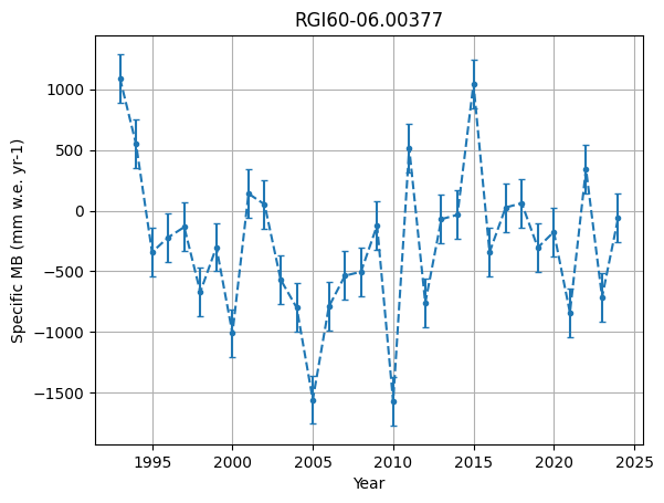
Apply CF Convention and Export as GeoZarr#
After creating the enhanced L1 data cube, we can update the metadata for all variables to follow the CF Convention using the DTCG API’s GeoZarrHandler.
from dtcg.datacube.geozarr import GeoZarrHandler

datacube_handler_aut = GeoZarrHandler(dtcg_oggm_aut.datacube_l1)

datacube_handler_aut.data_tree
<xarray.DataTree>
Group: /
└── Group: /L1
        Dimensions:                  (y: 229, x: 254, t_sfc_type: 82, snowcover_frac: 3)
        Coordinates:
          * y                        (y) float32 916B 5.199e+06 5.199e+06 ... 5.187e+06
          * x                        (x) float32 1kB 6.321e+05 6.322e+05 ... 6.45e+05
          * t_sfc_type               (t_sfc_type) int64 656B 1435968000 ... 1632528000
          * snowcover_frac           (snowcover_frac) float64 24B 0.25 0.5 0.75
            spatial_ref              int64 8B 0
        Data variables: (12/17)
            topo                     (y, x) float32 233kB 1.742e+03 ... 2.256e+03
            topo_smoothed            (y, x) float32 233kB 1.725e+03 ... 2.283e+03
            topo_valid_mask          (y, x) int8 58kB 1 1 1 1 1 1 1 1 ... 1 1 1 1 1 1 1
            glacier_mask             (y, x) int8 58kB 0 0 0 0 0 0 0 0 ... 0 0 0 0 0 0 0
            glacier_ext              (y, x) int8 58kB 0 0 0 0 0 0 0 0 ... 0 0 0 0 0 0 0
            consensus_ice_thickness  (y, x) float32 233kB nan nan nan ... nan nan nan
            ...                       ...
            millan_vx                (y, x) float32 233kB nan nan nan ... nan nan nan
            millan_vy                (y, x) float32 233kB nan nan nan ... nan nan nan
            hugonnet_dhdt            (y, x) float32 233kB 0.1893 0.1624 ... 0.001232
            sfc_type_data            (t_sfc_type, y, x) float64 38MB nan nan ... nan nan
            sfc_type_uncertainty     (t_sfc_type, y, x) float64 38MB nan nan ... nan nan
            sfc_type_snowline        (snowcover_frac, t_sfc_type) float64 2kB -inf .....
        Attributes:
            Conventions:         CF-1.12
            comment:             The DTC Glaciers project is developed under the Euro...
            date_created:        2026-02-24T16:42:51.963778
            RGI-ID:              RGI60-11.00719
            glacier_attributes:  {'rgi_id': 'RGI60-11.00719', 'glims_id': 'G010818E46...
            title:               Datacube of glacier-domain variables.
summary: Resampled glacier-domain variables from multiple sou...- y: 229
- x: 254
- t_sfc_type: 82
- snowcover_frac: 3
- y(y)float325.199e+06 5.199e+06 ... 5.187e+06
- units :
- m
- long_name :
- y coordinate of projection
- standard_name :
- projection_y_coordinate
array([5.198700e+06, 5.198648e+06, 5.198598e+06, ..., 5.187174e+06,5.187122e+06, 5.187072e+06], shape=(229,), dtype=float32)
- x(x)float326.321e+05 6.322e+05 ... 6.45e+05
- units :
- m
- long_name :
- x coordinate of projection
- standard_name :
- projection_x_coordinate
array([632125.5, 632176.5, 632227.5, ..., 644926.5, 644977.5, 645028.5],shape=(254,), dtype=float32)
- t_sfc_type(t_sfc_type)int641435968000 ... 1632528000
- long_name :
- time since the unix epoch of surface type observations
- standard_name :
- time
- units :
- seconds since 1970-01-01 00:00:00
array([1435968000, 1438560000, 1439424000, 1440547200, 1445472000, 1463875200,1467072000, 1468800000, 1470528000, 1472256000, 1473379200, 1474848000,1476576000, 1477699200, 1494979200, 1495843200, 1497312000, 1498435200,1499299200, 1500163200, 1501891200, 1502064000, 1503360000, 1503619200,1504051200, 1505952000, 1529107200, 1529712000, 1530403200, 1531440000,1531872000, 1532563200, 1532995200, 1534464000, 1534723200, 1535328000,1537315200, 1537488000, 1537920000, 1556755200, 1558656000, 1559347200,1559520000, 1560384000, 1560816000, 1561680000, 1563235200, 1563840000,1566864000, 1567123200, 1567555200, 1568592000, 1569024000, 1569715200,1590019200, 1591056000, 1591920000, 1593216000, 1594080000, 1594512000,1595808000, 1596240000, 1596672000, 1596931200, 1597104000, 1597795200,1597968000, 1599091200, 1599264000, 1599523200, 1599955200, 1600128000,1628640000, 1628899200, 1629504000, 1630627200, 1630800000, 1631232000,1631491200, 1631923200, 1632355200, 1632528000])
- snowcover_frac(snowcover_frac)float640.25 0.5 0.75
- long_name :
- Snowcover fraction of elevation band
- standard_name :
- snowcover_frac
- units :
- N/A
array([0.25, 0.5 , 0.75])
- spatial_ref()int640
- crs_wkt :
- PROJCS["unknown",GEOGCS["unknown",DATUM["WGS_1984",SPHEROID["WGS 84",6378137,298.257223563,AUTHORITY["EPSG","7030"]],AUTHORITY["EPSG","6326"]],PRIMEM["Greenwich",0,AUTHORITY["EPSG","8901"]],UNIT["degree",0.0174532925199433,AUTHORITY["EPSG","9122"]]],PROJECTION["Transverse_Mercator"],PARAMETER["latitude_of_origin",0],PARAMETER["central_meridian",9],PARAMETER["scale_factor",0.9996],PARAMETER["false_easting",500000],PARAMETER["false_northing",0],UNIT["metre",1,AUTHORITY["EPSG","9001"]],AXIS["Easting",EAST],AXIS["Northing",NORTH]]
- semi_major_axis :
- 6378137.0
- semi_minor_axis :
- 6356752.314245179
- inverse_flattening :
- 298.257223563
- reference_ellipsoid_name :
- WGS 84
- longitude_of_prime_meridian :
- 0.0
- prime_meridian_name :
- Greenwich
- geographic_crs_name :
- unknown
- horizontal_datum_name :
- World Geodetic System 1984
- projected_crs_name :
- unknown
- grid_mapping_name :
- transverse_mercator
- latitude_of_projection_origin :
- 0.0
- longitude_of_central_meridian :
- 9.0
- false_easting :
- 500000.0
- false_northing :
- 0.0
- scale_factor_at_central_meridian :
- 0.9996
- spatial_ref :
- PROJCS["unknown",GEOGCS["unknown",DATUM["WGS_1984",SPHEROID["WGS 84",6378137,298.257223563,AUTHORITY["EPSG","7030"]],AUTHORITY["EPSG","6326"]],PRIMEM["Greenwich",0,AUTHORITY["EPSG","8901"]],UNIT["degree",0.0174532925199433,AUTHORITY["EPSG","9122"]]],PROJECTION["Transverse_Mercator"],PARAMETER["latitude_of_origin",0],PARAMETER["central_meridian",9],PARAMETER["scale_factor",0.9996],PARAMETER["false_easting",500000],PARAMETER["false_northing",0],UNIT["metre",1,AUTHORITY["EPSG","9001"]],AXIS["Easting",EAST],AXIS["Northing",NORTH]]
array(0)
- topo(y, x)float321.742e+03 1.719e+03 ... 2.256e+03
- units :
- m
- long_name :
- Surface elevation from Copernicus DEM
- standard_name :
- surface_elevation
- institution :
- ESA / Copernicus Programme
- source :
- Observational - Copernicus DEM from Sentinel-1 and SRTM satellite data
- comment :
- Elevation data from Copernicus DEM (30m and 90m resolution), reprojected to glacier-specific grid. No-data values are set to NaN.
- references :
- https://doi.org/10.5270/ESA-c5d3d65
- grid_mapping :
- spatial_ref
array([[1742.0565, 1718.5181, 1704.2761, ..., 2634.5364, 2637.226 ,2649.449 ],[1740.664 , 1714.4333, 1704.7688, ..., 2638.1663, 2647.0886,2669.9976],[1736.8108, 1715.1503, 1707.2252, ..., 2642.6921, 2663.412 ,2690.577 ],...,[2751.1343, 2759.4119, 2786.9155, ..., 2333.323 , 2293.8684,2260.5007],[2716.279 , 2725.114 , 2737.6365, ..., 2320.2432, 2284.971 ,2255.3079],[2691.5476, 2701.3706, 2716.6023, ..., 2306.4504, 2277.612 ,2256.4653]], shape=(229, 254), dtype=float32)
- topo_smoothed(y, x)float321.725e+03 1.719e+03 ... 2.283e+03
- units :
- m
- long_name :
- Smoothed surface elevation from Copernicus DEM
- standard_name :
- surface_elevation_smoothed
- institution :
- ESA / Copernicus Programme, post-processed by OGGM
- source :
- Copernicus DEM data processed with Gaussian blur
- comment :
- Smoothed version of the Copernicus DEM using a Gaussian filter with user-defined window. Reprojected to glacier-specific grid.
- references :
- https://doi.org/10.5270/ESA-c5d3d65
- grid_mapping :
- spatial_ref
array([[1724.8086, 1719.3458, 1712.1177, ..., 2636.773 , 2646.762 ,2652.9497],[1724.4166, 1719.1144, 1712.0779, ..., 2641.2793, 2652.6218,2659.8135],[1724.0541, 1718.9253, 1712.0941, ..., 2649.7158, 2663.504 ,2672.4287],...,[2769.0166, 2785.2014, 2816.7178, ..., 2337.9739, 2310.3232,2294.3115],[2743.747 , 2758.433 , 2787.9717, ..., 2328.795 , 2302.123 ,2286.7192],[2729.0059, 2742.7756, 2771.012 , ..., 2323.2456, 2297.5151,2282.7017]], shape=(229, 254), dtype=float32)
- topo_valid_mask(y, x)int81 1 1 1 1 1 1 1 ... 1 1 1 1 1 1 1 1
- units :
- -
- long_name :
- Validity mask of Copernicus DEM surface elevation
- standard_name :
- surface_elevation_quality_flag
- institution :
- ESA / Copernicus Programme, post-processed by OGGM
- source :
- Validity mask derived from Copernicus DEM
- comment :
- 1 indicates valid DEM data; 0 indicates missing or invalid values.
- references :
- https://doi.org/10.5270/ESA-c5d3d65
- grid_mapping :
- spatial_ref
array([[1, 1, 1, ..., 1, 1, 1],[1, 1, 1, ..., 1, 1, 1],[1, 1, 1, ..., 1, 1, 1],...,[1, 1, 1, ..., 1, 1, 1],[1, 1, 1, ..., 1, 1, 1],[1, 1, 1, ..., 1, 1, 1]], shape=(229, 254), dtype=int8)
- glacier_mask(y, x)int80 0 0 0 0 0 0 0 ... 0 0 0 0 0 0 0 0
- units :
- -
- long_name :
- Glacier mask derived from Randolph Glacier Inventory (RGI v6)
- standard_name :
- ice_binary_mask
- institution :
- RGI Consortium
- source :
- Rasterized glacier extent from RGI. RGI definitions are manually and semi-automatically delineated glacier outlines from satellite imagery.
- comment :
- 1 indicates glacier-covered pixel; 0 indicates no ice.
- references :
- https://doi.org/10.7265/4m1f-gd79
- grid_mapping :
- spatial_ref
array([[0, 0, 0, ..., 0, 0, 0],[0, 0, 0, ..., 0, 0, 0],[0, 0, 0, ..., 0, 0, 0],...,[0, 0, 0, ..., 0, 0, 0],[0, 0, 0, ..., 0, 0, 0],[0, 0, 0, ..., 0, 0, 0]], shape=(229, 254), dtype=int8)
- glacier_ext(y, x)int80 0 0 0 0 0 0 0 ... 0 0 0 0 0 0 0 0
- units :
- -
- long_name :
- Glacier boundary derived from Randolph Glacier Inventory (RGI v6)
- standard_name :
- land_ice_boundary_binary_mask
- institution :
- RGI Consortium
- source :
- Rasterized glacier boundary from RGI. RGI definitions are manually and semi-automatically delineated glacier outlines from satellite imagery.
- comment :
- Marks the boundary pixels of the glacier outline, excluding nunataks.
- references :
- https://doi.org/10.7265/4m1f-gd79
- grid_mapping :
- spatial_ref
array([[0, 0, 0, ..., 0, 0, 0],[0, 0, 0, ..., 0, 0, 0],[0, 0, 0, ..., 0, 0, 0],...,[0, 0, 0, ..., 0, 0, 0],[0, 0, 0, ..., 0, 0, 0],[0, 0, 0, ..., 0, 0, 0]], shape=(229, 254), dtype=int8)
- consensus_ice_thickness(y, x)float32nan nan nan nan ... nan nan nan nan
- units :
- m
- long_name :
- Ice thickness from Farinotti et al. 2019 consensus estimate
- base_url :
- https://cluster.klima.uni-bremen.de/~fmaussion/icevol/composite/
- standard_name :
- consensus_ice_thickness
- institution :
- International consortium (ETH Zurich, WSL, University of Fribourg, et al.)
- source :
- Consensus estimate combining six glacier ice-thickness inversion models constrained by observations (Farinotti et al. 2019)
- comment :
- Ensemble-mean thickness resampled to the glacier-specific grid; represents estimates around the RGI v6 inventory epoch (~2000). Zero or negative values are masked to NaN.
- references :
- https://doi.org/10.1038/s41561-019-0300-3
- grid_mapping :
- spatial_ref
array([[nan, nan, nan, ..., nan, nan, nan],[nan, nan, nan, ..., nan, nan, nan],[nan, nan, nan, ..., nan, nan, nan],...,[nan, nan, nan, ..., nan, nan, nan],[nan, nan, nan, ..., nan, nan, nan],[nan, nan, nan, ..., nan, nan, nan]],shape=(229, 254), dtype=float32)
- itslive_v(y, x)float320.2434 0.2606 ... 0.2455 0.2186
- units :
- m yr-1
- long_name :
- Ice surface velocity magnitude from ITS_LIVE
- standard_name :
- ice_surface_velocity
- institution :
- NASA Jet Propulsion Laboratory (JPL), California Institute of Technology
- source :
- Observational - optical feature tracking of Landsat image pairs (ITS_LIVE composite, a NASA MEaSUREs project, its-live.jpl.nasa.gov)
- comment :
- Magnitude of the 1985-2018 average surface velocity, reprojected to glacier-specific grid and scaled to preserve ground units.
- references :
- https://doi.org/10.5067/6II6VW8LLWJ7
- grid_mapping :
- spatial_ref
array([[0.24344647, 0.26063082, 0.25035125, ..., 0.3579173 , 0.33561128,0.28883582],[0.215022 , 0.23906074, 0.23105459, ..., 0.23957004, 0.2915858 ,0.25415778],[0.2174102 , 0.22514711, 0.21218726, ..., 0.19214211, 0.23711233,0.22129242],...,[0.12075873, 0.10186059, 0.1240496 , ..., 0.38581932, 0.2984355 ,0.27908072],[0.12112405, 0.08944868, 0.11879443, ..., 0.3723072 , 0.2577669 ,0.24903257],[0.2777302 , 0.29464224, 0.36886322, ..., 0.32898155, 0.2455291 ,0.21862198]], shape=(229, 254), dtype=float32)
- itslive_vx(y, x)float320.1682 0.183 ... -0.02476 -0.05019
- units :
- m yr-1
- long_name :
- Ice surface velocity in x-direction from ITS_LIVE
- standard_name :
- ice_surface_x_velocity
- institution :
- NASA Jet Propulsion Laboratory (JPL), California Institute of Technology
- source :
- Observational - optical feature tracking of Landsat image pairs (ITS_LIVE composite, a NASA MEaSUREs project, its-live.jpl.nasa.gov)
- comment :
- x-component of 1985-2018 average surface velocity, reprojected to glacier-specific grid and scaled to preserve ground units.
- references :
- https://doi.org/10.5067/6II6VW8LLWJ7
- grid_mapping :
- spatial_ref
array([[ 0.16823728, 0.18299547, 0.21395968, ..., 0.14311485,0.18160792, 0.16164705],[ 0.21357566, 0.23756774, 0.23035474, ..., 0.23543918,0.28862417, 0.25171182],[ 0.2174102 , 0.22514711, 0.21218726, ..., 0.19214211,0.23711233, 0.22129242],...,[ 0.09323441, 0.05910604, 0.06591155, ..., -0.09302186,-0.16451906, -0.21805006],[ 0.06243233, 0.00519245, 0.00568864, ..., -0.12723948,-0.18808964, -0.2339943 ],[ 0.07564991, 0.05815558, 0.06371289, ..., -0.04651477,-0.02475613, -0.05019299]], shape=(229, 254), dtype=float32)
- itslive_vy(y, x)float32-0.09633 -0.09943 ... -0.05135 0.0
- units :
- m yr-1
- long_name :
- Ice surface velocity in y-direction from ITS_LIVE
- standard_name :
- ice_surface_y_velocity
- institution :
- NASA Jet Propulsion Laboratory (JPL), California Institute of Technology
- source :
- Observational - optical feature tracking of Landsat image pairs (ITS_LIVE composite, a NASA MEaSUREs project, its-live.jpl.nasa.gov)
- comment :
- y-component of 1985-2018 average surface velocity, reprojected to glacier-specific grid and scaled to preserve ground units.
- references :
- https://doi.org/10.5067/6II6VW8LLWJ7
- grid_mapping :
- spatial_ref
array([[-0.09632614, -0.09943351, -0.04660948, ..., -0.22293597,-0.16981854, -0.14407717],[-0.00185245, -0.0019122 , -0.00089635, ..., -0.00428728,-0.00326578, -0.00277075],[ 0. , 0. , 0. , ..., 0. ,0. , 0. ],...,[ 0. , 0. , 0. , ..., -0.31767195,-0.16941534, -0.08806729],[-0.01928749, -0.02240353, -0.02785993, ..., -0.26921242,-0.06118476, 0. ],[-0.2160203 , -0.25092 , -0.3120319 , ..., -0.2259387 ,-0.0513498 , 0. ]], shape=(229, 254), dtype=float32)
- millan_ice_thickness(y, x)float32nan nan nan nan ... nan nan nan nan
- units :
- m
- long_name :
- Ice thickness from Millan et al. 2022
- data_source :
- RGI-11_2021July09
- standard_name :
- millan_ice_thickness
- institution :
- University of California, Irvine; CNRS / IGE; University Grenoble Alpes
- source :
- Mass-conservation inversion constrained by multi-mission surface velocities and surface mass balance (Millan et al. 2022)
- comment :
- Ice thickness estimated from mass-conservation inversion using multi-mission velocity mosaics (SAR/optical, ~2000-2018) and SMB; reprojected to glacier-specific grid. Zero or negative values masked to NaN.
- references :
- https://doi.org/10.1038/s41561-021-00885-z
- grid_mapping :
- spatial_ref
array([[nan, nan, nan, ..., nan, nan, nan],[nan, nan, nan, ..., nan, nan, nan],[nan, nan, nan, ..., nan, nan, nan],...,[nan, nan, nan, ..., nan, nan, nan],[nan, nan, nan, ..., nan, nan, nan],[nan, nan, nan, ..., nan, nan, nan]],shape=(229, 254), dtype=float32)
- millan_v(y, x)float32nan nan nan nan ... nan nan nan nan
- units :
- m yr-1
- long_name :
- Ice surface velocity magnitude from Millan et al. 2022
- data_source :
- RGI-11_2021July01
- standard_name :
- millan_ice_surface_velocity
- institution :
- University of California, Irvine; CNRS / IGE; University Grenoble Alpes
- source :
- Multi-mission surface velocity mosaic from SAR and optical feature tracking (Sentinel-1, Landsat-8, TerraSAR-X/TanDEM-X, ALOS)
- comment :
- Multi-year (~2000-2018) average surface velocity magnitude, reprojected to glacier-specific grid; resampled to preserve ground units.
- references :
- https://doi.org/10.1038/s41561-021-00885-z
- grid_mapping :
- spatial_ref
array([[nan, nan, nan, ..., nan, nan, nan],[nan, nan, nan, ..., nan, nan, nan],[nan, nan, nan, ..., nan, nan, nan],...,[nan, nan, nan, ..., nan, nan, nan],[nan, nan, nan, ..., nan, nan, nan],[nan, nan, nan, ..., nan, nan, nan]],shape=(229, 254), dtype=float32)
- millan_vx(y, x)float32nan nan nan nan ... nan nan nan nan
- units :
- m yr-1
- long_name :
- Ice surface velocity in x-direction from Millan et al. 2022
- data_source :
- RGI-11_2021July01
- standard_name :
- millan_ice_surface_x_velocity
- institution :
- University of California, Irvine; CNRS / IGE; University Grenoble Alpes
- source :
- Multi-mission surface velocity mosaic from SAR and optical feature tracking (Sentinel-1, Landsat-8, TerraSAR-X/TanDEM-X, ALOS)
- comment :
- Multi-year (~2000-2018) average x-component of surface velocity, reprojected to glacier-specific grid; resampled to preserve ground units.
- references :
- https://doi.org/10.1038/s41561-021-00885-z
- grid_mapping :
- spatial_ref
array([[nan, nan, nan, ..., nan, nan, nan],[nan, nan, nan, ..., nan, nan, nan],[nan, nan, nan, ..., nan, nan, nan],...,[nan, nan, nan, ..., nan, nan, nan],[nan, nan, nan, ..., nan, nan, nan],[nan, nan, nan, ..., nan, nan, nan]],shape=(229, 254), dtype=float32)
- millan_vy(y, x)float32nan nan nan nan ... nan nan nan nan
- units :
- m yr-1
- long_name :
- Ice surface velocity in y-direction from Millan et al. 2022
- data_source :
- RGI-11_2021July01
- standard_name :
- millan_ice_surface_y_velocity
- institution :
- University of California, Irvine; CNRS / IGE; University Grenoble Alpes
- source :
- Multi-mission surface velocity mosaic from SAR and optical feature tracking (Sentinel-1, Landsat-8, TerraSAR-X/TanDEM-X, ALOS)
- comment :
- Multi-year (~2000-2018) average y-component of surface velocity, reprojected to glacier-specific grid; resampled to preserve ground units.
- references :
- https://doi.org/10.1038/s41561-021-00885-z
- grid_mapping :
- spatial_ref
array([[nan, nan, nan, ..., nan, nan, nan],[nan, nan, nan, ..., nan, nan, nan],[nan, nan, nan, ..., nan, nan, nan],...,[nan, nan, nan, ..., nan, nan, nan],[nan, nan, nan, ..., nan, nan, nan],[nan, nan, nan, ..., nan, nan, nan]],shape=(229, 254), dtype=float32)
- hugonnet_dhdt(y, x)float320.1893 0.1624 ... 0.004438 0.001232
- units :
- m yr-1
- long_name :
- Glacier elevation change rate from geodetic mass balance estimates
- data_source :
- /home/data/download/cluster.klima.uni-bremen.de/~oggm/geodetic_ref_mb_maps/dhdt/N46E010_2000-01-01_2020-01-01_dhdt.tif
- standard_name :
- ice_elevation_change_rate
- institution :
- ETH Zurich / University of Toulouse / University of Oslo
- source :
- Geodetic measurements from multi-temporal DEMs (optical stereo from ASTER)
- comment :
- Rate of surface elevation change (dh/dt) derived for 2000-2019; reprojected to the glacier-specific grid. Values outside data coverage remain NaN.
- references :
- https://www.nature.com/articles/s41586-021-03436-z
- grid_mapping :
- spatial_ref
array([[ 1.8931952e-01, 1.6242915e-01, 1.4414129e-01, ...,-1.1726944e+00, -8.4028047e-01, -5.2263099e-01],[ 1.9792432e-01, 1.8828717e-01, 3.7784296e-01, ...,-1.0144438e+00, -6.3453114e-01, -3.5095587e-01],[ 2.0982631e-01, 2.2902362e-01, 6.1095959e-01, ...,-8.5337508e-01, -4.3152189e-01, -1.8335494e-01],...,[-8.4933359e-03, -2.2932557e-02, -2.3965480e-02, ...,-7.7997725e-03, -7.1713943e-03, -5.7778261e-03],[-3.8133018e-02, -3.8725853e-02, -2.9151555e-02, ...,-9.8316406e-04, 4.3411115e-03, 3.5339131e-03],[-6.1521191e-02, -7.7394404e-02, -6.3811660e-02, ...,-1.6706563e-04, 4.4379705e-03, 1.2322172e-03]],shape=(229, 254), dtype=float32)
- sfc_type_data(t_sfc_type, y, x)float64nan nan nan nan ... nan nan nan nan
- long_name :
- Glacier surface type classification from Sentinel-2
- data_source :
- ENVEO
- units :
- -
- code_description :
- Extract dict with eval(ds.code).
- code :
- {0: 'unclassified', 1: 'snow', 2: 'firn / old snow / bright ice', 3: 'clean ice', 4: 'debris', 5: 'cloud', 'nan': 'no data'}
- standard_name :
- glacier_surface_classification
- institution :
- ENVEO
- source :
- Spectral classification of Sentinel-2 multi-spectral imagery (10m) using threshold-based method with 6S radiative transfer model and CAMS atmospheric parameters (Cremona et al. 2025)
- comment :
- Classification of glacier surface facies derived from Sentinel-2 scenes (2015-23, <15% cloud cover). Classes include snow, clean glacier ice, debris-covered ice, and firn/old snow/bright ice (seasonal). Reprojected to glacier-specific grid.
- references :
- https://doi.org/10.1017/jog.2025.1
- grid_mapping :
- spatial_ref
array([[[nan, nan, nan, ..., nan, nan, nan],[nan, nan, nan, ..., nan, nan, nan],[nan, nan, nan, ..., nan, nan, nan],...,[nan, nan, nan, ..., nan, nan, nan],[nan, nan, nan, ..., nan, nan, nan],[nan, nan, nan, ..., nan, nan, nan]],[[nan, nan, nan, ..., nan, nan, nan],[nan, nan, nan, ..., nan, nan, nan],[nan, nan, nan, ..., nan, nan, nan],...,[nan, nan, nan, ..., nan, nan, nan],[nan, nan, nan, ..., nan, nan, nan],[nan, nan, nan, ..., nan, nan, nan]],[[nan, nan, nan, ..., nan, nan, nan],[nan, nan, nan, ..., nan, nan, nan],[nan, nan, nan, ..., nan, nan, nan],...,......,[nan, nan, nan, ..., nan, nan, nan],[nan, nan, nan, ..., nan, nan, nan],[nan, nan, nan, ..., nan, nan, nan]],[[nan, nan, nan, ..., nan, nan, nan],[nan, nan, nan, ..., nan, nan, nan],[nan, nan, nan, ..., nan, nan, nan],...,[nan, nan, nan, ..., nan, nan, nan],[nan, nan, nan, ..., nan, nan, nan],[nan, nan, nan, ..., nan, nan, nan]],[[nan, nan, nan, ..., nan, nan, nan],[nan, nan, nan, ..., nan, nan, nan],[nan, nan, nan, ..., nan, nan, nan],...,[nan, nan, nan, ..., nan, nan, nan],[nan, nan, nan, ..., nan, nan, nan],[nan, nan, nan, ..., nan, nan, nan]]], shape=(82, 229, 254))
- sfc_type_uncertainty(t_sfc_type, y, x)float64nan nan nan nan ... nan nan nan nan
- long_name :
- Uncertainty in glacier surface type classification from Sentinel-2
- data_source :
- ENVEO
- units :
- -
- code_description :
- Extract dict with eval(ds.code).
- code :
- {1: 'low uncertainty for illuminated pixel', 2: 'medium uncertainty for illuminated pixel', 3: 'high uncertainty for illuminated pixel', 5: 'cloud', 11: 'low uncertainty for shaded pixel', 12: 'medium uncertainty for shaded pixel', 13: 'high uncertainty for shaded pixel', 'nan': 'no data'}
- standard_name :
- glacier_surface_classification_uncertainty
- institution :
- ENVEO
- source :
- Uncertainty estimates from spectral classification algorithm (Cremona et al. 2025)
- comment :
- Estimated classification uncertainty in surface facies determination. Based on spectral reflectance thresholds and reclassification scheme.
- references :
- https://doi.org/10.1017/jog.2025.1
- grid_mapping :
- spatial_ref
array([[[nan, nan, nan, ..., nan, nan, nan],[nan, nan, nan, ..., nan, nan, nan],[nan, nan, nan, ..., nan, nan, nan],...,[nan, nan, nan, ..., nan, nan, nan],[nan, nan, nan, ..., nan, nan, nan],[nan, nan, nan, ..., nan, nan, nan]],[[nan, nan, nan, ..., nan, nan, nan],[nan, nan, nan, ..., nan, nan, nan],[nan, nan, nan, ..., nan, nan, nan],...,[nan, nan, nan, ..., nan, nan, nan],[nan, nan, nan, ..., nan, nan, nan],[nan, nan, nan, ..., nan, nan, nan]],[[nan, nan, nan, ..., nan, nan, nan],[nan, nan, nan, ..., nan, nan, nan],[nan, nan, nan, ..., nan, nan, nan],...,......,[nan, nan, nan, ..., nan, nan, nan],[nan, nan, nan, ..., nan, nan, nan],[nan, nan, nan, ..., nan, nan, nan]],[[nan, nan, nan, ..., nan, nan, nan],[nan, nan, nan, ..., nan, nan, nan],[nan, nan, nan, ..., nan, nan, nan],...,[nan, nan, nan, ..., nan, nan, nan],[nan, nan, nan, ..., nan, nan, nan],[nan, nan, nan, ..., nan, nan, nan]],[[nan, nan, nan, ..., nan, nan, nan],[nan, nan, nan, ..., nan, nan, nan],[nan, nan, nan, ..., nan, nan, nan],...,[nan, nan, nan, ..., nan, nan, nan],[nan, nan, nan, ..., nan, nan, nan],[nan, nan, nan, ..., nan, nan, nan]]], shape=(82, 229, 254))
- sfc_type_snowline(snowcover_frac, t_sfc_type)float64-inf 3.09e+03 ... nan 3.09e+03
- long_name :
- Snowline altitude from Sentinel-2 surface classification
- data_source :
- ENVEO
- units :
- m
- inf_values :
- {inf: 3570.0, -inf: 2760.0}
- standard_name :
- equilibrium_line_altitude
- institution :
- ENVEO
- source :
- Snowline derived from snow-covered area fraction (SCAF) computed from surface type classification (Cremona et al. 2025)
- comment :
- Altitude of snowline (transient equilibrium line) determined from snow-covered area fraction derived via surface type classification. Represents the boundary between snow and firn/ice/debris on the glacier surface; computed from Sentinel-2 facies classification (2015-23).
- references :
- https://doi.org/10.1017/jog.2025.1
array([[ -inf, 3090., 3120., 3180., -inf, -inf, -inf, -inf, -inf,3120., 2880., -inf, -inf, -inf, -inf, -inf, -inf, -inf,3000., 2970., 3270., 3120., 3090., 3390., inf, -inf, -inf,-inf, nan, 3000., 3030., nan, 3120., 3240., 3120., -inf,3390., 3420., 3420., -inf, -inf, -inf, -inf, -inf, -inf,-inf, 2880., -inf, 3180., 3360., 3240., 2940., 3180., 2910.,-inf, -inf, -inf, -inf, -inf, 2880., 3000., 3030., 2910.,3060., 3090., 3090., 3120., 2910., 3090., 3090., 3240., 3240.,nan, 3120., 3120., nan, 2940., 3000., 3120., 3180., nan,2940.],[ -inf, 3120., 3210., 3240., -inf, -inf, -inf, -inf, -inf,3240., 2910., -inf, -inf, -inf, -inf, -inf, -inf, 3000.,3030., 3000., inf, 3180., 3120., inf, inf, -inf, -inf,-inf, nan, 3030., 3060., nan, 3210., inf, inf, 2940.,3390., 3420., inf, -inf, -inf, -inf, -inf, -inf, -inf,-inf, 2880., 2880., 3240., inf, 3420., 3000., 3270., 2940.,-inf, -inf, -inf, -inf, 2880., 2940., 3030., 3090., 2940.,3090., 3120., 3120., 3240., 2940., 3120., 3120., 3420., 3420.,nan, 3180., 3180., nan, 3000., 3090., 3180., 3240., nan,2970.],[ -inf, 3210., 3420., 3390., -inf, -inf, -inf, -inf, -inf,3420., inf, -inf, -inf, -inf, -inf, -inf, -inf, 3030.,3060., 3060., inf, 3180., 3180., inf, inf, -inf, -inf,-inf, nan, 3060., 3090., nan, 3300., inf, inf, 2970.,3420., inf, inf, -inf, -inf, -inf, -inf, -inf, -inf,-inf, 2940., 2970., 3420., inf, 3420., 3090., 3420., 2940.,-inf, -inf, -inf, -inf, 2940., 2940., 3060., 3120., 2940.,3240., 3390., 3420., 3420., 2940., 3240., 3150., 3420., 3450.,nan, 3240., 3270., nan, 3060., 3120., 3270., 3390., nan,3090.]])
- Conventions :
- CF-1.12
- comment :
- The DTC Glaciers project is developed under the European Space Agency's Digital Twin Earth initiative, as part of the Digital Twin Components (DTC) Early Development Actions.
- date_created :
- 2026-02-24T16:42:51.963778
- RGI-ID :
- RGI60-11.00719
- glacier_attributes :
- {'rgi_id': 'RGI60-11.00719', 'glims_id': 'G010818E46876N', 'cenlon': 10.818, 'cenlat': 46.8762, 'rgi_region': '11', 'rgi_subregion': '11-01', 'rgi_version': '60', 'rgi_dem_source': 'COPDEM30', 'glacier_type': 'Glacier', 'terminus_type': 'Land-terminating', 'name': 'Vernagtferner', 'rgi_region_name': '11: Central Europe', 'rgi_subregion_name': '11-01: Alps ', 'rgi_date': 2003}
- title :
- Datacube of glacier-domain variables.
- summary :
- Resampled glacier-domain variables from multiple sources for RGI6-ID 'RGI60-11.00719'. Generated for the DTC Glaciers project.

from pathlib import Path
import tempfile

with tempfile.TemporaryDirectory(suffix=".zarr") as tmpdir:
    output_path = Path(tmpdir)
    datacube_handler_aut.export(output_path)
    print(f"✅ GeoZarr exported to: {output_path}")
    items = sorted(p.name for p in output_path.iterdir())
    print("📂 Top-level contents:", ", ".join(items) or "(empty)")
✅ GeoZarr exported to: /tmp/tmp1huz1sxk.zarr
📂 Top-level contents: .zattrs, .zgroup, .zmetadata, L1
Preprocessed data cubes for case study regions#
Preprocessed L1 data cubes, including all currently supported observations, are available for the case study regions in Iceland and Austria. You can obtain the URL of the latest version via DEFAULT_L1_DATACUBE_URL and use the DTCG API’s dedicated data cube streaming functionality as shown below:
from dtcg import DEFAULT_L1_DATACUBE_URL
from dtcg.api.external.call import StreamDatacube

streamer = StreamDatacube(server=DEFAULT_L1_DATACUBE_URL)
datacube = streamer.stream_datacube(glacier=rgi_id_ice)
datacube
<xarray.DataTree>
Group: /
└── Group: /L1
        Dimensions:                                  (y: 370, x: 436, t: 177, t_wgms: 32)
        Coordinates:
          * y                                        (y) float32 1kB 7.201e+06 ... 7....
          * x                                        (x) float32 2kB 3.94e+05 ... 4.8...
          * t                                        (t) datetime64[ns] 1kB 2011-01-1...
          * t_wgms                                   (t_wgms) int64 256B 1993 ... 2024
        Data variables: (12/21)
            consensus_ice_thickness                  (y, x) float32 645kB dask.array<chunksize=(370, 436), meta=np.ndarray>
            eolis_elevation_change_sigma_timeseries  (t) float64 1kB dask.array<chunksize=(177,), meta=np.ndarray>
            eolis_elevation_change_timeseries        (t) float64 1kB dask.array<chunksize=(177,), meta=np.ndarray>
            eolis_gridded_elevation_change           (t, y, x) float64 228MB dask.array<chunksize=(177, 60, 60), meta=np.ndarray>
            eolis_gridded_elevation_change_sigma     (t, y, x) float64 228MB dask.array<chunksize=(177, 60, 60), meta=np.ndarray>
            glacier_ext                              (y, x) int8 161kB dask.array<chunksize=(370, 436), meta=np.ndarray>
            ...                                       ...
            spatial_ref                              int64 8B ...
            topo                                     (y, x) float32 645kB dask.array<chunksize=(370, 436), meta=np.ndarray>
            topo_smoothed                            (y, x) float32 645kB dask.array<chunksize=(370, 436), meta=np.ndarray>
            topo_valid_mask                          (y, x) int8 161kB dask.array<chunksize=(370, 436), meta=np.ndarray>
            wgms_mb                                  (t_wgms) float64 256B dask.array<chunksize=(32,), meta=np.ndarray>
            wgms_mb_unc                              (t_wgms) float64 256B dask.array<chunksize=(32,), meta=np.ndarray>
        Attributes:
            Conventions:         CF-1.12
            comment:             The DTC Glaciers project is developed under the Euro...
            date_created:        2026-01-10T23:48:41.290684
            RGI-ID:              RGI60-06.00377
            glacier_attributes:  {'rgi_id': 'RGI60-06.00377', 'glims_id': 'G343733E64...
            title:               Datacube of glacier-domain variables.
summary: Resampled glacier-domain variables from multiple sou...- y: 370
- x: 436
- t: 177
- t_wgms: 32
- y(y)float327.201e+06 7.201e+06 ... 7.127e+06
- units :
- m
- long_name :
- y coordinate of projection
- standard_name :
- projection_y_coordinate
array([7.200982e+06, 7.200782e+06, 7.200582e+06, ..., 7.127582e+06,7.127382e+06, 7.127182e+06], shape=(370,), dtype=float32)
- x(x)float323.94e+05 3.942e+05 ... 4.81e+05
- units :
- m
- long_name :
- x coordinate of projection
- standard_name :
- projection_x_coordinate
array([393962.1, 394162.1, 394362.1, ..., 480562.1, 480762.1, 480962.1],shape=(436,), dtype=float32)
- t(t)datetime64[ns]2011-01-15 ... 2025-09-15
- standard_name :
- time
- long_name :
- time since the unix epoch of eolis observations
array(['2011-01-15T00:00:00.000000000', '2011-02-15T00:00:00.000000000','2011-03-15T00:00:00.000000000', '2011-04-15T00:00:00.000000000','2011-05-15T00:00:00.000000000', '2011-06-15T00:00:00.000000000','2011-07-15T00:00:00.000000000', '2011-08-15T00:00:00.000000000','2011-09-15T00:00:00.000000000', '2011-10-15T00:00:00.000000000','2011-11-15T00:00:00.000000000', '2011-12-15T00:00:00.000000000','2012-01-15T00:00:00.000000000', '2012-02-15T00:00:00.000000000','2012-03-15T00:00:00.000000000', '2012-04-15T00:00:00.000000000','2012-05-15T00:00:00.000000000', '2012-06-15T00:00:00.000000000','2012-07-15T00:00:00.000000000', '2012-08-15T00:00:00.000000000','2012-09-15T00:00:00.000000000', '2012-10-15T00:00:00.000000000','2012-11-15T00:00:00.000000000', '2012-12-15T00:00:00.000000000','2013-01-15T00:00:00.000000000', '2013-02-15T00:00:00.000000000','2013-03-15T00:00:00.000000000', '2013-04-15T00:00:00.000000000','2013-05-15T00:00:00.000000000', '2013-06-15T00:00:00.000000000','2013-07-15T00:00:00.000000000', '2013-08-15T00:00:00.000000000','2013-09-15T00:00:00.000000000', '2013-10-15T00:00:00.000000000','2013-11-15T00:00:00.000000000', '2013-12-15T00:00:00.000000000','2014-01-15T00:00:00.000000000', '2014-02-15T00:00:00.000000000','2014-03-15T00:00:00.000000000', '2014-04-15T00:00:00.000000000','2014-05-15T00:00:00.000000000', '2014-06-15T00:00:00.000000000','2014-07-15T00:00:00.000000000', '2014-08-15T00:00:00.000000000','2014-09-15T00:00:00.000000000', '2014-10-15T00:00:00.000000000','2014-11-15T00:00:00.000000000', '2014-12-15T00:00:00.000000000','2015-01-15T00:00:00.000000000', '2015-02-15T00:00:00.000000000','2015-03-15T00:00:00.000000000', '2015-04-15T00:00:00.000000000','2015-05-15T00:00:00.000000000', '2015-06-15T00:00:00.000000000','2015-07-15T00:00:00.000000000', '2015-08-15T00:00:00.000000000','2015-09-15T00:00:00.000000000', '2015-10-15T00:00:00.000000000','2015-11-15T00:00:00.000000000', '2015-12-15T00:00:00.000000000','2016-01-15T00:00:00.000000000', '2016-02-15T00:00:00.000000000','2016-03-15T00:00:00.000000000', '2016-04-15T00:00:00.000000000','2016-05-15T00:00:00.000000000', '2016-06-15T00:00:00.000000000','2016-07-15T00:00:00.000000000', '2016-08-15T00:00:00.000000000','2016-09-15T00:00:00.000000000', '2016-10-15T00:00:00.000000000','2016-11-15T00:00:00.000000000', '2016-12-15T00:00:00.000000000','2017-01-15T00:00:00.000000000', '2017-02-15T00:00:00.000000000','2017-03-15T00:00:00.000000000', '2017-04-15T00:00:00.000000000','2017-05-15T00:00:00.000000000', '2017-06-15T00:00:00.000000000','2017-07-15T00:00:00.000000000', '2017-08-15T00:00:00.000000000','2017-09-15T00:00:00.000000000', '2017-10-15T00:00:00.000000000','2017-11-15T00:00:00.000000000', '2017-12-15T00:00:00.000000000','2018-01-15T00:00:00.000000000', '2018-02-15T00:00:00.000000000','2018-03-15T00:00:00.000000000', '2018-04-15T00:00:00.000000000','2018-05-15T00:00:00.000000000', '2018-06-15T00:00:00.000000000','2018-07-15T00:00:00.000000000', '2018-08-15T00:00:00.000000000','2018-09-15T00:00:00.000000000', '2018-10-15T00:00:00.000000000','2018-11-15T00:00:00.000000000', '2018-12-15T00:00:00.000000000','2019-01-15T00:00:00.000000000', '2019-02-15T00:00:00.000000000','2019-03-15T00:00:00.000000000', '2019-04-15T00:00:00.000000000','2019-05-15T00:00:00.000000000', '2019-06-15T00:00:00.000000000','2019-07-15T00:00:00.000000000', '2019-08-15T00:00:00.000000000','2019-09-15T00:00:00.000000000', '2019-10-15T00:00:00.000000000','2019-11-15T00:00:00.000000000', '2019-12-15T00:00:00.000000000','2020-01-15T00:00:00.000000000', '2020-02-15T00:00:00.000000000','2020-03-15T00:00:00.000000000', '2020-04-15T00:00:00.000000000','2020-05-15T00:00:00.000000000', '2020-06-15T00:00:00.000000000','2020-07-15T00:00:00.000000000', '2020-08-15T00:00:00.000000000','2020-09-15T00:00:00.000000000', '2020-10-15T00:00:00.000000000','2020-11-15T00:00:00.000000000', '2020-12-15T00:00:00.000000000','2021-01-15T00:00:00.000000000', '2021-02-15T00:00:00.000000000','2021-03-15T00:00:00.000000000', '2021-04-15T00:00:00.000000000','2021-05-15T00:00:00.000000000', '2021-06-15T00:00:00.000000000','2021-07-15T00:00:00.000000000', '2021-08-15T00:00:00.000000000','2021-09-15T00:00:00.000000000', '2021-10-15T00:00:00.000000000','2021-11-15T00:00:00.000000000', '2021-12-15T00:00:00.000000000','2022-01-15T00:00:00.000000000', '2022-02-15T00:00:00.000000000','2022-03-15T00:00:00.000000000', '2022-04-15T00:00:00.000000000','2022-05-15T00:00:00.000000000', '2022-06-15T00:00:00.000000000','2022-07-15T00:00:00.000000000', '2022-08-15T00:00:00.000000000','2022-09-15T00:00:00.000000000', '2022-10-15T00:00:00.000000000','2022-11-15T00:00:00.000000000', '2022-12-15T00:00:00.000000000','2023-01-15T00:00:00.000000000', '2023-02-15T00:00:00.000000000','2023-03-15T00:00:00.000000000', '2023-04-15T00:00:00.000000000','2023-05-15T00:00:00.000000000', '2023-06-15T00:00:00.000000000','2023-07-15T00:00:00.000000000', '2023-08-15T00:00:00.000000000','2023-09-15T00:00:00.000000000', '2023-10-15T00:00:00.000000000','2023-11-15T00:00:00.000000000', '2023-12-15T00:00:00.000000000','2024-01-15T00:00:00.000000000', '2024-02-15T00:00:00.000000000','2024-03-15T00:00:00.000000000', '2024-04-15T00:00:00.000000000','2024-05-15T00:00:00.000000000', '2024-06-15T00:00:00.000000000','2024-07-15T00:00:00.000000000', '2024-08-15T00:00:00.000000000','2024-09-15T00:00:00.000000000', '2024-10-15T00:00:00.000000000','2024-11-15T00:00:00.000000000', '2024-12-15T00:00:00.000000000','2025-01-15T00:00:00.000000000', '2025-02-15T00:00:00.000000000','2025-03-15T00:00:00.000000000', '2025-04-15T00:00:00.000000000','2025-05-15T00:00:00.000000000', '2025-06-15T00:00:00.000000000','2025-07-15T00:00:00.000000000', '2025-08-15T00:00:00.000000000','2025-09-15T00:00:00.000000000'], dtype='datetime64[ns]')
- t_wgms(t_wgms)int641993 1994 1995 ... 2022 2023 2024
- standard_name :
- time
- long_name :
- the hydrological year of WGMS observations
- units :
- year
array([1993, 1994, 1995, 1996, 1997, 1998, 1999, 2000, 2001, 2002, 2003, 2004,2005, 2006, 2007, 2008, 2009, 2010, 2011, 2012, 2013, 2014, 2015, 2016,2017, 2018, 2019, 2020, 2021, 2022, 2023, 2024])
- consensus_ice_thickness(y, x)float32dask.array<chunksize=(370, 436), meta=np.ndarray>
- units :
- m
- long_name :
- Ice thickness from Farinotti et al. 2019 consensus estimate
- base_url :
- https://cluster.klima.uni-bremen.de/~fmaussion/icevol/composite/
- standard_name :
- consensus_ice_thickness
- institution :
- International consortium (ETH Zurich, WSL, University of Fribourg, et al.)
- source :
- Consensus estimate combining six glacier ice-thickness inversion models constrained by observations (Farinotti et al. 2019)
- comment :
- Ensemble-mean thickness resampled to the glacier-specific grid; represents estimates around the RGI v6 inventory epoch (~2000). Zero or negative values are masked to NaN.
- references :
- https://doi.org/10.1038/s41561-019-0300-3
- grid_mapping :
- spatial_ref
Array Chunk Bytes 630.16 kiB 630.16 kiB Shape (370, 436) (370, 436) Dask graph 1 chunks in 2 graph layers Data type float32 numpy.ndarray - eolis_elevation_change_sigma_timeseries(t)float64dask.array<chunksize=(177,), meta=np.ndarray>
- units :
- m
- comment :
- Uncertainty propagated using a static 20 km spatial correlation length.
- institution :
- Earthwave/The University of Edinburgh/ESA
- long_name :
- Uncertainty of change in land-ice surface altitude since January 2011
- references :
- EOLIS elevation data generated using swath processing of CryoSat-2 data (Jakob & Gourmelen, 2023) and provided by the ESA CryoTEMPO project (https://cryotempo-eolis.org/). Jakob, L., and Gourmelen, N., (2023). Glacier Mass Loss Between 2010 and 2020 Dominated by Atmospheric Forcing. Geophysical Research Letters 50(8), 1-10. doi:10.1029/2023GL102954
- source :
- Observed cells: CryoTEMPO-EOLIS uncertainties; interpolated cells: GPR predictive standard deviation.Values represent propagated 1-sigma uncertainty of the glacier-wide mean, estimated from pixel-level uncertainties (eolis_gridded_elevation_change_sigma) using a spatial correlation model.
- standard_name :
- change_over_time_in_land_ice_surface_altitude_standard_error
- ancillary_variables :
- eolis_elevation_change_timeseries
Array Chunk Bytes 1.38 kiB 1.38 kiB Shape (177,) (177,) Dask graph 1 chunks in 2 graph layers Data type float64 numpy.ndarray - eolis_elevation_change_timeseries(t)float64dask.array<chunksize=(177,), meta=np.ndarray>
- units :
- m
- ancillary_variables :
- eolis_elevation_change_sigma_timeseries
- comment :
- Computed from eolis_gridded_elevation_change. Elevation change since January 2011.
- institution :
- Earthwave/The University of Edinburgh/ESA
- long_name :
- change in land-ice surface altitude since January 2011
- references :
- EOLIS elevation data generated using swath processing of CryoSat-2 data (Jakob & Gourmelen, 2023) and provided by the ESA CryoTEMPO project (https://cryotempo-eolis.org/). Jakob, L., and Gourmelen, N., (2023). Glacier Mass Loss Between 2010 and 2020 Dominated by Atmospheric Forcing. Geophysical Research Letters 50(8), 1-10. doi:10.1029/2023GL102954
- source :
- CryoTEMPO-EOLIS gridded product; gaps filled with GPR. Observed values retained; only missing cells interpolated.Values represent glacier-wide mean elevation change, computed as the average of all valid grid cells (eolis_gridded_elevation_change) within the glacier mask.
- standard_name :
- change_over_time_in_land_ice_surface_altitude
Array Chunk Bytes 1.38 kiB 1.38 kiB Shape (177,) (177,) Dask graph 1 chunks in 2 graph layers Data type float64 numpy.ndarray - eolis_gridded_elevation_change(t, y, x)float64dask.array<chunksize=(177, 60, 60), meta=np.ndarray>
- units :
- m
- ancillary_variables :
- elevation_change_sigma, interpolation_binary_mask
- comment :
- Elevation change since January 2011.
- institution :
- Earthwave/The University of Edinburgh/ESA
- long_name :
- change in land-ice surface altitude since January 2011
- references :
- EOLIS elevation data generated using swath processing of CryoSat-2 data (Jakob & Gourmelen, 2023) and provided by the ESA CryoTEMPO project (https://cryotempo-eolis.org/). Jakob, L., and Gourmelen, N., (2023). Glacier Mass Loss Between 2010 and 2020 Dominated by Atmospheric Forcing. Geophysical Research Letters 50(8), 1-10. doi:10.1029/2023GL102954
- source :
- CryoTEMPO-EOLIS gridded product; gaps filled with GPR. Observed values retained; only missing cells interpolated.
- standard_name :
- change_over_time_in_land_ice_surface_altitude
- grid_mapping :
- spatial_ref
Array Chunk Bytes 217.85 MiB 4.86 MiB Shape (177, 370, 436) (177, 60, 60) Dask graph 56 chunks in 2 graph layers Data type float64 numpy.ndarray - eolis_gridded_elevation_change_sigma(t, y, x)float64dask.array<chunksize=(177, 60, 60), meta=np.ndarray>
- units :
- m
- comment :
- Mixture of observational and GPR uncertainties, aligned to elevation_change.
- institution :
- Earthwave/The University of Edinburgh/ESA
- long_name :
- Uncertainty of change in land-ice surface altitude since January 2011
- references :
- EOLIS elevation data generated using swath processing of CryoSat-2 data (Jakob & Gourmelen, 2023) and provided by the ESA CryoTEMPO project (https://cryotempo-eolis.org/). Jakob, L., and Gourmelen, N., (2023). Glacier Mass Loss Between 2010 and 2020 Dominated by Atmospheric Forcing. Geophysical Research Letters 50(8), 1-10. doi:10.1029/2023GL102954
- source :
- Observed cells: CryoTEMPO-EOLIS uncertainties; interpolated cells: GPR predictive standard deviation.
- standard_name :
- change_over_time_in_land_ice_surface_altitude_standard_error
- grid_mapping :
- spatial_ref
Array Chunk Bytes 217.85 MiB 4.86 MiB Shape (177, 370, 436) (177, 60, 60) Dask graph 56 chunks in 2 graph layers Data type float64 numpy.ndarray - glacier_ext(y, x)int8dask.array<chunksize=(370, 436), meta=np.ndarray>
- units :
- -
- long_name :
- Glacier boundary derived from Randolph Glacier Inventory (RGI v6)
- standard_name :
- land_ice_boundary_binary_mask
- institution :
- RGI Consortium
- source :
- Rasterized glacier boundary from RGI. RGI definitions are manually and semi-automatically delineated glacier outlines from satellite imagery.
- comment :
- Marks the boundary pixels of the glacier outline, excluding nunataks.
- references :
- https://doi.org/10.7265/4m1f-gd79
- grid_mapping :
- spatial_ref
Array Chunk Bytes 157.54 kiB 157.54 kiB Shape (370, 436) (370, 436) Dask graph 1 chunks in 2 graph layers Data type int8 numpy.ndarray - glacier_mask(y, x)int8dask.array<chunksize=(370, 436), meta=np.ndarray>
- units :
- -
- long_name :
- Glacier mask derived from Randolph Glacier Inventory (RGI v6)
- standard_name :
- ice_binary_mask
- institution :
- RGI Consortium
- source :
- Rasterized glacier extent from RGI. RGI definitions are manually and semi-automatically delineated glacier outlines from satellite imagery.
- comment :
- 1 indicates glacier-covered pixel; 0 indicates no ice.
- references :
- https://doi.org/10.7265/4m1f-gd79
- grid_mapping :
- spatial_ref
Array Chunk Bytes 157.54 kiB 157.54 kiB Shape (370, 436) (370, 436) Dask graph 1 chunks in 2 graph layers Data type int8 numpy.ndarray - hugonnet_dhdt(y, x)float32dask.array<chunksize=(370, 436), meta=np.ndarray>
- units :
- m yr-1
- long_name :
- Glacier elevation change rate from geodetic mass balance estimates
- data_source :
- /home/data/download/cluster.klima.uni-bremen.de/~oggm/geodetic_ref_mb_maps/dhdt/N64W017_2000-01-01_2020-01-01_dhdt.tif /home/data/download/cluster.klima.uni-bremen.de/~oggm/geodetic_ref_mb_maps/dhdt/N64W016_2000-01-01_2020-01-01_dhdt.tif
- standard_name :
- ice_elevation_change_rate
- institution :
- ETH Zurich / University of Toulouse / University of Oslo
- source :
- Geodetic measurements from multi-temporal DEMs (optical stereo from ASTER)
- comment :
- Rate of surface elevation change (dh/dt) derived for 2000-2019; reprojected to the glacier-specific grid. Values outside data coverage remain NaN.
- references :
- https://www.nature.com/articles/s41586-021-03436-z
- grid_mapping :
- spatial_ref
Array Chunk Bytes 630.16 kiB 630.16 kiB Shape (370, 436) (370, 436) Dask graph 1 chunks in 2 graph layers Data type float32 numpy.ndarray - itslive_v(y, x)float32dask.array<chunksize=(370, 436), meta=np.ndarray>
- units :
- m yr-1
- long_name :
- Ice surface velocity magnitude from ITS_LIVE
- standard_name :
- ice_surface_velocity
- institution :
- NASA Jet Propulsion Laboratory (JPL), California Institute of Technology
- source :
- Observational - optical feature tracking of Landsat image pairs (ITS_LIVE composite, a NASA MEaSUREs project, its-live.jpl.nasa.gov)
- comment :
- Magnitude of the 1985-2018 average surface velocity, reprojected to glacier-specific grid and scaled to preserve ground units.
- references :
- https://doi.org/10.5067/6II6VW8LLWJ7
- grid_mapping :
- spatial_ref
Array Chunk Bytes 630.16 kiB 630.16 kiB Shape (370, 436) (370, 436) Dask graph 1 chunks in 2 graph layers Data type float32 numpy.ndarray - itslive_vx(y, x)float32dask.array<chunksize=(370, 436), meta=np.ndarray>
- units :
- m yr-1
- long_name :
- Ice surface velocity in x-direction from ITS_LIVE
- standard_name :
- ice_surface_x_velocity
- institution :
- NASA Jet Propulsion Laboratory (JPL), California Institute of Technology
- source :
- Observational - optical feature tracking of Landsat image pairs (ITS_LIVE composite, a NASA MEaSUREs project, its-live.jpl.nasa.gov)
- comment :
- x-component of 1985-2018 average surface velocity, reprojected to glacier-specific grid and scaled to preserve ground units.
- references :
- https://doi.org/10.5067/6II6VW8LLWJ7
- grid_mapping :
- spatial_ref
Array Chunk Bytes 630.16 kiB 630.16 kiB Shape (370, 436) (370, 436) Dask graph 1 chunks in 2 graph layers Data type float32 numpy.ndarray - itslive_vy(y, x)float32dask.array<chunksize=(370, 436), meta=np.ndarray>
- units :
- m yr-1
- long_name :
- Ice surface velocity in y-direction from ITS_LIVE
- standard_name :
- ice_surface_y_velocity
- institution :
- NASA Jet Propulsion Laboratory (JPL), California Institute of Technology
- source :
- Observational - optical feature tracking of Landsat image pairs (ITS_LIVE composite, a NASA MEaSUREs project, its-live.jpl.nasa.gov)
- comment :
- y-component of 1985-2018 average surface velocity, reprojected to glacier-specific grid and scaled to preserve ground units.
- references :
- https://doi.org/10.5067/6II6VW8LLWJ7
- grid_mapping :
- spatial_ref
Array Chunk Bytes 630.16 kiB 630.16 kiB Shape (370, 436) (370, 436) Dask graph 1 chunks in 2 graph layers Data type float32 numpy.ndarray - millan_ice_thickness(y, x)float32dask.array<chunksize=(370, 436), meta=np.ndarray>
- units :
- m
- long_name :
- Ice thickness from Millan et al. 2022
- data_source :
- RGI-6_2021July09
- standard_name :
- millan_ice_thickness
- institution :
- University of California, Irvine; CNRS / IGE; University Grenoble Alpes
- source :
- Mass-conservation inversion constrained by multi-mission surface velocities and surface mass balance (Millan et al. 2022)
- comment :
- Ice thickness estimated from mass-conservation inversion using multi-mission velocity mosaics (SAR/optical, ~2000-2018) and SMB; reprojected to glacier-specific grid. Zero or negative values masked to NaN.
- references :
- https://doi.org/10.1038/s41561-021-00885-z
- grid_mapping :
- spatial_ref
Array Chunk Bytes 630.16 kiB 630.16 kiB Shape (370, 436) (370, 436) Dask graph 1 chunks in 2 graph layers Data type float32 numpy.ndarray - millan_v(y, x)float32dask.array<chunksize=(370, 436), meta=np.ndarray>
- units :
- m yr-1
- long_name :
- Ice surface velocity magnitude from Millan et al. 2022
- data_source :
- RGI-6_2021July01
- standard_name :
- millan_ice_surface_velocity
- institution :
- University of California, Irvine; CNRS / IGE; University Grenoble Alpes
- source :
- Multi-mission surface velocity mosaic from SAR and optical feature tracking (Sentinel-1, Landsat-8, TerraSAR-X/TanDEM-X, ALOS)
- comment :
- Multi-year (~2000-2018) average surface velocity magnitude, reprojected to glacier-specific grid; resampled to preserve ground units.
- references :
- https://doi.org/10.1038/s41561-021-00885-z
- grid_mapping :
- spatial_ref
Array Chunk Bytes 630.16 kiB 630.16 kiB Shape (370, 436) (370, 436) Dask graph 1 chunks in 2 graph layers Data type float32 numpy.ndarray - millan_vx(y, x)float32dask.array<chunksize=(370, 436), meta=np.ndarray>
- units :
- m yr-1
- long_name :
- Ice surface velocity in x-direction from Millan et al. 2022
- data_source :
- RGI-6_2021July01
- standard_name :
- millan_ice_surface_x_velocity
- institution :
- University of California, Irvine; CNRS / IGE; University Grenoble Alpes
- source :
- Multi-mission surface velocity mosaic from SAR and optical feature tracking (Sentinel-1, Landsat-8, TerraSAR-X/TanDEM-X, ALOS)
- comment :
- Multi-year (~2000-2018) average x-component of surface velocity, reprojected to glacier-specific grid; resampled to preserve ground units.
- references :
- https://doi.org/10.1038/s41561-021-00885-z
- grid_mapping :
- spatial_ref
Array Chunk Bytes 630.16 kiB 630.16 kiB Shape (370, 436) (370, 436) Dask graph 1 chunks in 2 graph layers Data type float32 numpy.ndarray - millan_vy(y, x)float32dask.array<chunksize=(370, 436), meta=np.ndarray>
- units :
- m yr-1
- long_name :
- Ice surface velocity in y-direction from Millan et al. 2022
- data_source :
- RGI-6_2021July01
- standard_name :
- millan_ice_surface_y_velocity
- institution :
- University of California, Irvine; CNRS / IGE; University Grenoble Alpes
- source :
- Multi-mission surface velocity mosaic from SAR and optical feature tracking (Sentinel-1, Landsat-8, TerraSAR-X/TanDEM-X, ALOS)
- comment :
- Multi-year (~2000-2018) average y-component of surface velocity, reprojected to glacier-specific grid; resampled to preserve ground units.
- references :
- https://doi.org/10.1038/s41561-021-00885-z
- grid_mapping :
- spatial_ref
Array Chunk Bytes 630.16 kiB 630.16 kiB Shape (370, 436) (370, 436) Dask graph 1 chunks in 2 graph layers Data type float32 numpy.ndarray - spatial_ref()int64...
- crs_wkt :
- PROJCS["unknown",GEOGCS["unknown",DATUM["WGS_1984",SPHEROID["WGS 84",6378137,298.257223563,AUTHORITY["EPSG","7030"]],AUTHORITY["EPSG","6326"]],PRIMEM["Greenwich",0,AUTHORITY["EPSG","8901"]],UNIT["degree",0.0174532925199433,AUTHORITY["EPSG","9122"]]],PROJECTION["Transverse_Mercator"],PARAMETER["latitude_of_origin",0],PARAMETER["central_meridian",-15],PARAMETER["scale_factor",0.9996],PARAMETER["false_easting",500000],PARAMETER["false_northing",0],UNIT["metre",1,AUTHORITY["EPSG","9001"]],AXIS["Easting",EAST],AXIS["Northing",NORTH]]
- semi_major_axis :
- 6378137.0
- semi_minor_axis :
- 6356752.314245179
- inverse_flattening :
- 298.257223563
- reference_ellipsoid_name :
- WGS 84
- longitude_of_prime_meridian :
- 0.0
- prime_meridian_name :
- Greenwich
- geographic_crs_name :
- unknown
- horizontal_datum_name :
- World Geodetic System 1984
- projected_crs_name :
- unknown
- grid_mapping_name :
- transverse_mercator
- latitude_of_projection_origin :
- 0.0
- longitude_of_central_meridian :
- -15.0
- false_easting :
- 500000.0
- false_northing :
- 0.0
- scale_factor_at_central_meridian :
- 0.9996
- spatial_ref :
- PROJCS["unknown",GEOGCS["unknown",DATUM["WGS_1984",SPHEROID["WGS 84",6378137,298.257223563,AUTHORITY["EPSG","7030"]],AUTHORITY["EPSG","6326"]],PRIMEM["Greenwich",0,AUTHORITY["EPSG","8901"]],UNIT["degree",0.0174532925199433,AUTHORITY["EPSG","9122"]]],PROJECTION["Transverse_Mercator"],PARAMETER["latitude_of_origin",0],PARAMETER["central_meridian",-15],PARAMETER["scale_factor",0.9996],PARAMETER["false_easting",500000],PARAMETER["false_northing",0],UNIT["metre",1,AUTHORITY["EPSG","9001"]],AXIS["Easting",EAST],AXIS["Northing",NORTH]]
[1 values with dtype=int64]
- topo(y, x)float32dask.array<chunksize=(370, 436), meta=np.ndarray>
- units :
- m
- long_name :
- Surface elevation from Copernicus DEM
- standard_name :
- surface_elevation
- institution :
- ESA / Copernicus Programme
- source :
- Observational - Copernicus DEM from Sentinel-1 and SRTM satellite data
- comment :
- Elevation data from Copernicus DEM (30m and 90m resolution), reprojected to glacier-specific grid. No-data values are set to NaN.
- references :
- https://doi.org/10.5270/ESA-c5d3d65
- grid_mapping :
- spatial_ref
Array Chunk Bytes 630.16 kiB 630.16 kiB Shape (370, 436) (370, 436) Dask graph 1 chunks in 2 graph layers Data type float32 numpy.ndarray - topo_smoothed(y, x)float32dask.array<chunksize=(370, 436), meta=np.ndarray>
- units :
- m
- long_name :
- Smoothed surface elevation from Copernicus DEM
- standard_name :
- surface_elevation_smoothed
- institution :
- ESA / Copernicus Programme, post-processed by OGGM
- source :
- Copernicus DEM data processed with Gaussian blur
- comment :
- Smoothed version of the Copernicus DEM using a Gaussian filter with user-defined window. Reprojected to glacier-specific grid.
- references :
- https://doi.org/10.5270/ESA-c5d3d65
- grid_mapping :
- spatial_ref
Array Chunk Bytes 630.16 kiB 630.16 kiB Shape (370, 436) (370, 436) Dask graph 1 chunks in 2 graph layers Data type float32 numpy.ndarray - topo_valid_mask(y, x)int8dask.array<chunksize=(370, 436), meta=np.ndarray>
- units :
- -
- long_name :
- Validity mask of Copernicus DEM surface elevation
- standard_name :
- surface_elevation_quality_flag
- institution :
- ESA / Copernicus Programme, post-processed by OGGM
- source :
- Validity mask derived from Copernicus DEM
- comment :
- 1 indicates valid DEM data; 0 indicates missing or invalid values.
- references :
- https://doi.org/10.5270/ESA-c5d3d65
- grid_mapping :
- spatial_ref
Array Chunk Bytes 157.54 kiB 157.54 kiB Shape (370, 436) (370, 436) Dask graph 1 chunks in 2 graph layers Data type int8 numpy.ndarray - wgms_mb(t_wgms)float64dask.array<chunksize=(32,), meta=np.ndarray>
- units :
- kg m-2 yr-1
- source :
- In-situ measurements from glaciological surveys
- standard_name :
- specific_surface_mass_balance
- long_name :
- Glacier-wide specific mass balance from WGMS observations
- institution :
- World Glacier Monitoring Service (WGMS)
- comment :
- Annual specific (area-weighted) mass balance observations compiled by WGMS from direct glaciological measurements at monitored glaciers.
- references :
- https://doi.org/10.5904/wgms-fog-2023-12
Array Chunk Bytes 256 B 256 B Shape (32,) (32,) Dask graph 1 chunks in 2 graph layers Data type float64 numpy.ndarray - wgms_mb_unc(t_wgms)float64dask.array<chunksize=(32,), meta=np.ndarray>
- units :
- kg m-2 yr-1
- source :
- Uncertainty estimates from WGMS measurements
- standard_name :
- specific_surface_mass_balance_uncertainty
- long_name :
- Uncertainty in glacier-wide specific mass balance from WGMS
- institution :
- World Glacier Monitoring Service (WGMS)
- comment :
- Estimated uncertainty in annual specific mass balance, accounting for measurement and interpolation errors in WGMS observations.
- references :
- https://doi.org/10.5904/wgms-fog-2023-12
Array Chunk Bytes 256 B 256 B Shape (32,) (32,) Dask graph 1 chunks in 2 graph layers Data type float64 numpy.ndarray
- Conventions :
- CF-1.12
- comment :
- The DTC Glaciers project is developed under the European Space Agency's Digital Twin Earth initiative, as part of the Digital Twin Components (DTC) Early Development Actions.
- date_created :
- 2026-01-10T23:48:41.290684
- RGI-ID :
- RGI60-06.00377
- glacier_attributes :
- {'rgi_id': 'RGI60-06.00377', 'glims_id': 'G343733E64587N', 'cenlon': -16.2675, 'cenlat': 64.5867, 'rgi_region': '06', 'rgi_subregion': '06-01', 'rgi_version': '60', 'rgi_dem_source': 'COPDEM90', 'glacier_type': 'Ice cap', 'terminus_type': 'Land-terminating', 'name': 'Bruarjoekull', 'rgi_region_name': '06: Iceland', 'rgi_subregion_name': '06-01: Iceland ', 'rgi_date': 2000}
- title :
- Datacube of glacier-domain variables.
- summary :
- Resampled glacier-domain variables from multiple sources for RGI6-ID 'RGI60-06.00377'. Generated for the DTC Glaciers project.
Or you can use xr.open_datatree for data streaming:
def get_l1_data_tree(rgi_id):
    return xr.open_datatree(
        f"{DEFAULT_L1_DATACUBE_URL}{rgi_id}.zarr",
        chunks={},
        engine="zarr",
        consolidated=True,
        decode_cf=True,
    )
Streaming means that only a view of the available data, together with the corresponding coordinates, is provided first. The actual data are only downloaded when needed. This approach saves bandwidth and makes it fast to explore large datasets.
The preprocessed data cubes (L1 and L2, explained in this notebook) are currently available for all RGI6 glaciers of Vatnajökull (view in OpenStreetMap):
Show code cell source
Hide code cell source
from oggm import utils
import yaml
import geopandas as gpd
import seaborn as sns

sns.set_style("whitegrid")
sns.set_context("notebook")

dtcf_url = (
    "https://cluster.klima.uni-bremen.de/~dtcg/test_files/case_study_regions/iceland/"
)
with open(
    utils.file_downloader(dtcf_url + "vatnajokull_rgi_ids.yml"), "r"
) as yaml_file:
    rgi_ids = yaml.safe_load(yaml_file)["rgi_ids"]

# Select the outlines from RGI6 file and convert to UTM
rgi_file = gpd.read_file(utils.get_rgi_region_file("06"))
rgi_file = rgi_file.loc[rgi_file.RGIId.isin(rgi_ids)].set_index("RGIId")
rgi_file = rgi_file.to_crs("EPSG:32628")

rgi_file.plot(ec="k");
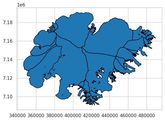
And for the Ötztal region in the Austrian Alps (view in OpenStreetMap):
Show code cell source
Hide code cell source
import json

dtcf_url = (
    "https://cluster.klima.uni-bremen.de/~dtcg/test_files/case_study_regions/austria/"
)
with open(utils.file_downloader(dtcf_url + "oeztal_rgi_ids.json"), "r") as json_file:
    rgi_ids = json.load(json_file)

# Select the outlines from RGI6 file and convert to UTM
rgi_file = gpd.read_file(utils.get_rgi_region_file("11"))
rgi_file = rgi_file.loc[rgi_file.RGIId.isin(rgi_ids)].set_index("RGIId")
rgi_file = rgi_file.to_crs("EPSG:32628")

rgi_file.plot(ec="k");
To obtain the RGI6 ID of a glacier, you can use the GLIMS Viewer. Enable the RGIv6 IDs in the menu in the top-right corner, zoom to the glacier of interest, and click on its outline to display the metadata.